Can an automated trading strategy outperform Bitcoin (BTC) and Ether (ETH) buy-and-hold “diamond hands"? We explore how to develop a simple automated trading strategy and what kind of performance we can expect out of it.
This post is longer than 30 minutes to read.
Preface
In this post, we explore how to develop a crude technical indicator-based trading strategy, and how far we can get with simple automated trading. The goal is not to create the best trading strategy in the world. Instead, we explore the process itself, including
- Explaining the benefits and trade-offs of systematic trading
- What does the process of developing an automated trading strategy look like?
- What are the trade-offs when considering risk vs. reward?
- How to develop your automated trading strategy
Trading idea
Everything begins with an idea. Ideas for an automated trading strategy can come from, for example
- Hands-on experience: manual trading and understanding the market behaviour by learning with experience.
- Literature: School books and studying trading strategies. See the Learning section in Trading Strategy documentation.
In this blog post, we follow the latter approach. We take an existing trading idea, see how we can tweak it, what kind of performance we can get out of it, and how to adopt it to DeFi markets.
Specifically, we explore the usage of the Relative Strength Indicator (RSI) in cryptocurrency momentum trading.
The hypothesis goes like this
- Cryptocurrency markets are momentum driven
- RSI can be used to detect this momentum purely based on price behaviour: The sentiment is visible in medium- and long-term price action
- By entering positions during the upward momentum and exiting when the momentum dries up, we can outperform a buy-and-hold strategy
This approach aims to codify and automate the decisions an experienced trader would make by manually analysing price action.
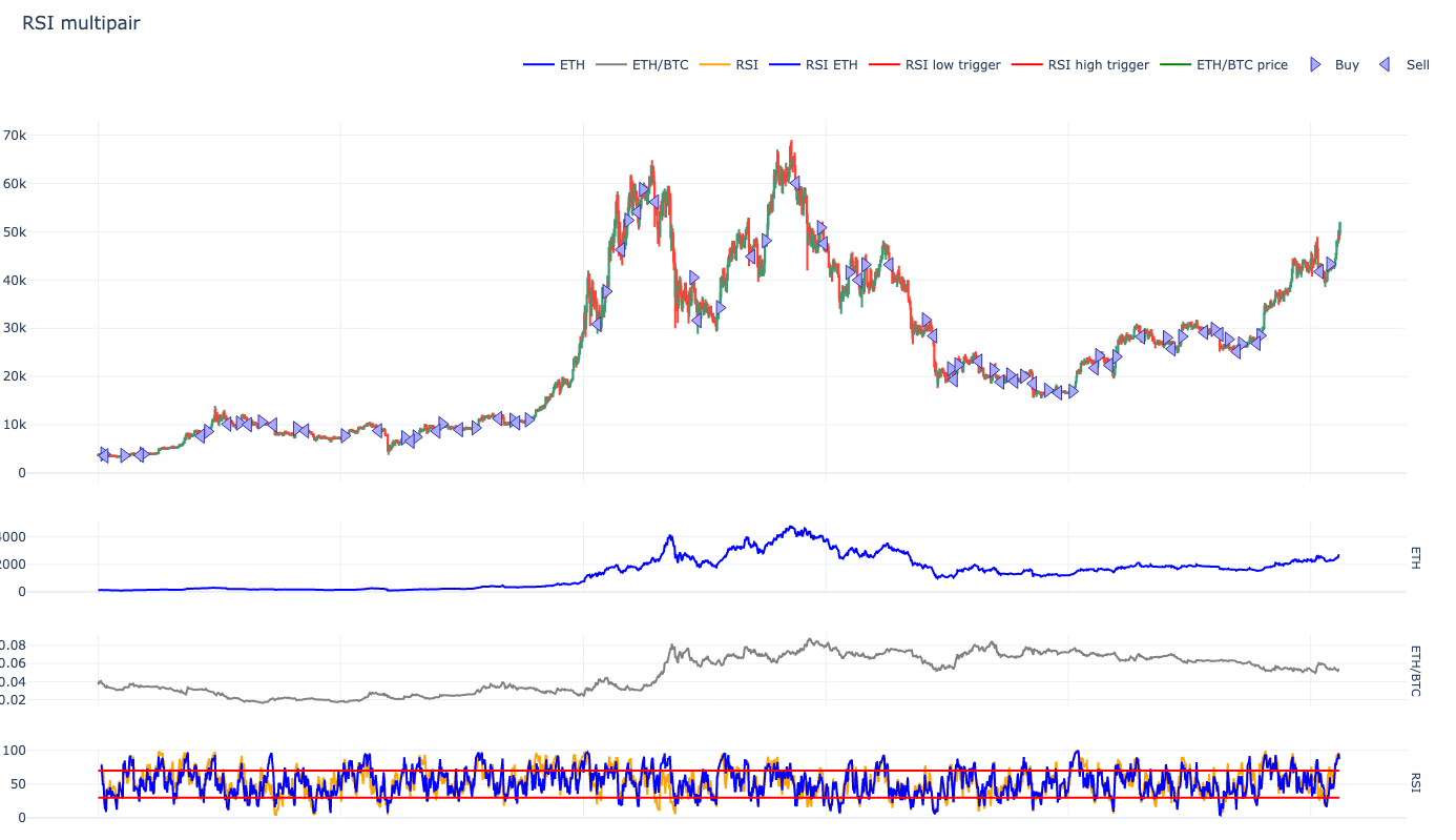
What is RSI?
The strategy is simplified—we only use a single technical indicator, RSI, calculated from the close of price candles. Thus, we need to understand what RSI means.
For a given time frame (length as number of price candles), RSI takes average time frame (usually daily) gains and losses and normalises this to a number between 0-100, adjusted to the volatility.
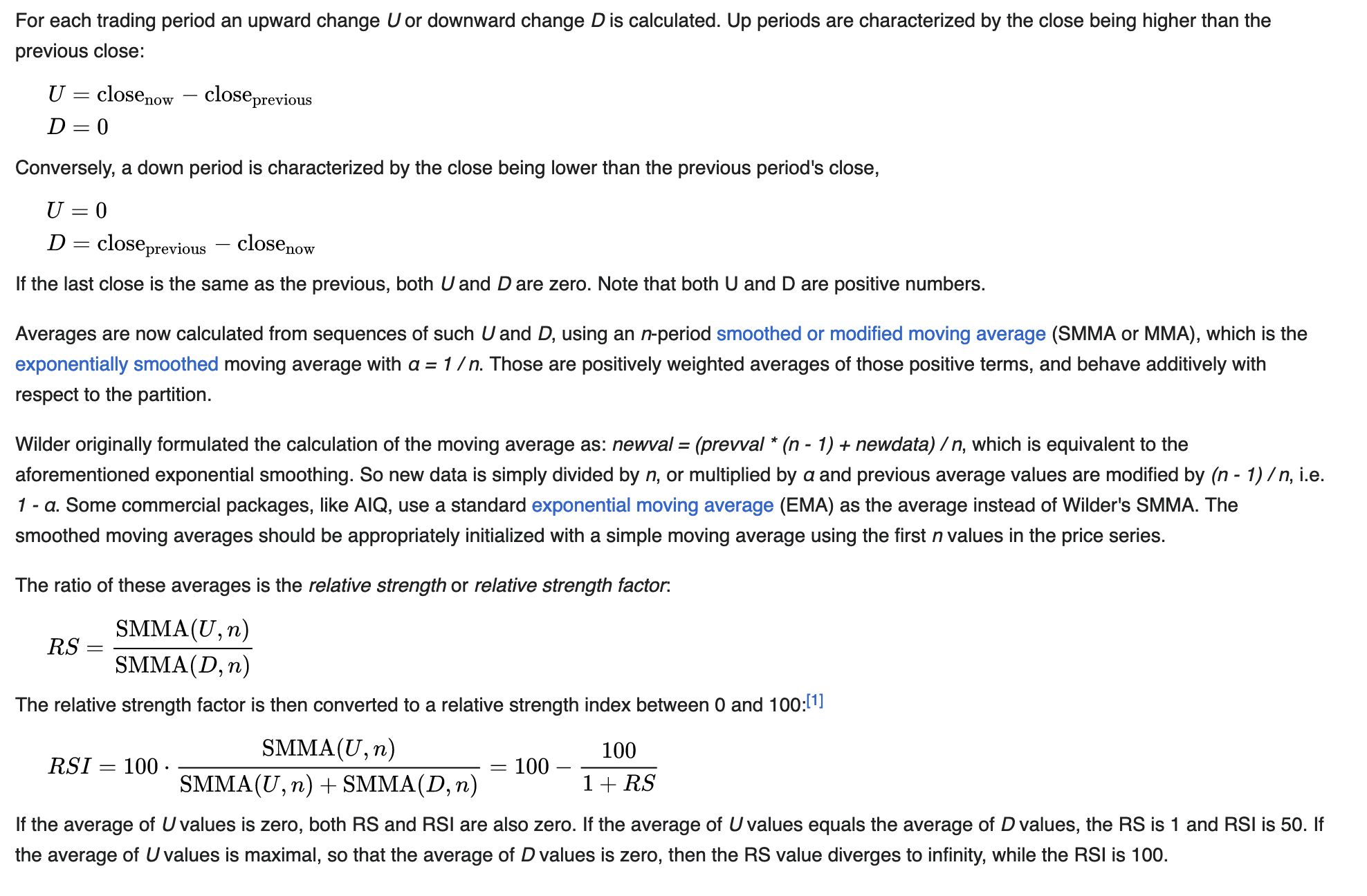
Assuming we take RSI of length 14 over the daily price candle close value:
- 100 = Infinite gains on every last 14 days
- 70 = Large daily gains (e.g. 5% daily on volatile markets, 1-2% daily gains on stable markets)
- 30 = Large daily losses
- 0 = infinite losses on every last 14 days
For traditional markets, an RSI value over 70 means “overbought” (should come down soon) and an RSI below 30 means “oversold” (should start to pick up and return to mean).
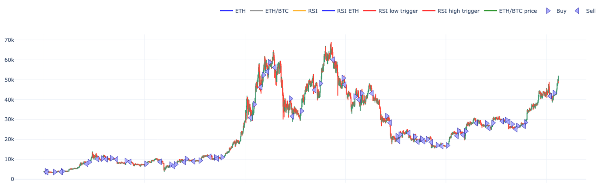
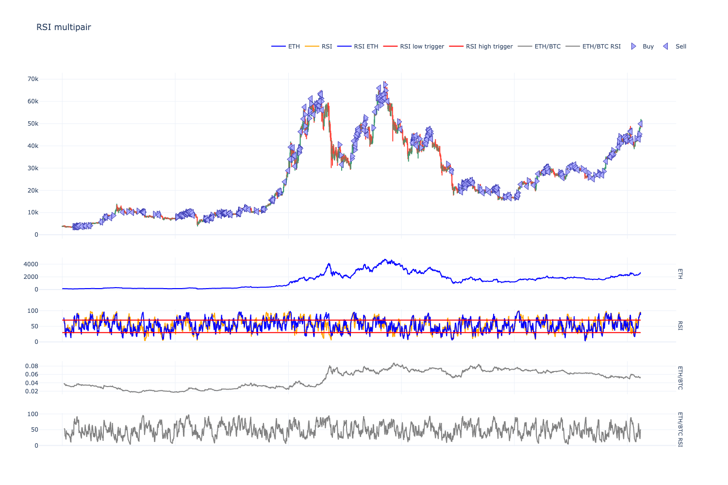
RSI is often plotted under the price chart as a separate chart. Here is an example chart.
RSI is a momentum indicator. In our strategy, instead of using a trend-reversing strategy (buy when it is oversold, sell when it is overbought), we will use the exact opposite (buy when others are buying, sell when others are selling). When it’s time to panic, it pays to be the first one out from the door, and because we are using automated trading, we expect this to be one of the key factors in the strategy's performance. Diamond hands will be left sitting on their losses.
Strategy plan
To keep it simple, we apply the following constraints:
- Market-taking strategy: we buy low and sell high, using market orders. The simplest trading there is.
- Spot only: We are going to do a spot-only trading strategy. Leveraged and shorting-enabled strategies are more profitable, but we operate with an extra constraint: we want to create a strategy that works with any DeFi digital asset management protocol and its vaults. Currently, a DeFi vault protocol supporting multi-vault owner leveraged positions does not exist (with a caveat: Hyperliquid supports this, but currently, Hyperliquid is centralised and closed source).
- No interest for USDC: We are also not taking advantage of any potential to accrue interest while not in the markets. We could do this, for example, by using the Aave stablecoin interest pool. This would improve the strategy's performance during high-interest rate years.
- BTC and ETH trading pairs only: Two trading pairs and cash is the most primitive portfolio construction strategy. Having more than one option to buy is always better, as we will find out shortly.
- 1-day and 8-hour time frames: We explore both daily candles and eight-hour candles.
Pros
Some benefits of this strategy.
- Simple to understand: anyone with trading experience and little software development experience can study and audit the strategy.
- Simple to implement: Using only one technical indicator means the fewest possible moving parts.
- Transparent and auditable: Because the strategy is simple and lacks any machine learning magic, it’s easy to understand why certain trades were made and what effects the performance.
- Trade with size: Both BTC and ETH are very liquid trading pairs. Today, BTC is likely one of the top 5 most liquid assets in the world. This means you need to worry less about fees, price impact, and scaling.
- Simple risk management: When trading spot only, one cannot get liquidated. Maximum capital at risk is at the level where the price falls under the RSI exit threshold. We also explore explicitly setting stop loss parameters.
- Never sleep: We use eight-hour candles. This is something a manual trader could not accomplish. There are advantages to deciding trades 24/7. Eight hours is a compromise between daily and hourly candles, since trading on a lower time frame significantly alters the market dynamics change a lot and trading becomes much more fee-sensitive.
- Mid-frequency trading: Rebalancing every eight hours is far from high-frequency trading, making the trade execution simpler.
Cons
- Up only: The spot-only strategy can only make money in an up-trend market. In a bear market, the strategy reserves cash or bleeds it slowly.
- Limited opportunities: there are approximately 10,000 cryptocurrencies or tokens, and we artificially limit ourselves to trade two.
- Unoptimal performance: By later exploring equity curves of different strategy outcomes, we can see that there are low-hanging fruit to improve the performance of this trading strategy with regime filters, additional indicators and so on.
- Static parameters: There is no feedback loop to adjust the parameters for market conditions like bull and bear markets (often called market regimes). We use the same RSI threshold values for BTC and ETH, even though we see that it might be beneficial to have per-pair thresholds due to their different price action characteristics.
Benchmarks and definitions of outperformance
When we compare the strategy, both to our internal variants and external opportunities, we call this benchmarking. We can roughly classify the steps to success as follows:
- Not losing money
- Outperforming USD risk-free rate
- Outperforming BTC
- Outperforming ETH, risk-adjusted
- Outperforming ETH, both risk-adjusted and absolute
- Outperforming ETH in a bull market
- Outperforming everything
The first step (1) is not to lose money. While it sounds obvious, without proper risk management, one could be easily liquidated with leveraged trades. With high leverage you might get liquidated on your average crypto bull market pullback day.
Next, you want to beat the US treasury notes (2). The US treasury note yield is what the world usually knows as the “risk-free” rate. Technically, it is not risk-free, as the piling up of US national debt increases the risk every day, but it is still less risky than everything else. You can get this "risk-free" in DeFi by parking your money, e.g., in the Aave USDC pool.
The first volatile trading goal is to outperform BTC (3). This does not need a strategy but can be achieved with buy-and-hold ETH, so we do not explore this much.
Then, we want to outperform ETH in a risk-adjusted manner (4). Here, risk-adjusted means that our portfolio's maximum drawdown is less than the maximum drawdown of buy-and-hold ETH, even if we end up with less profit. The usual way to compare risk-adjusted portfolio performance is the Sharpe ratio, although more is needed to get a whole picture.
After outperforming ETH in a risk-adjusted manner, we can move to absolute outperformance (5). This means we outperform diamond hands with less drawdown. We end up with a more valuable portfolio with less risk taken.
But we are not done yet. As one of Trading Strategy’s advisors once said, “All I want for Christmas is to outperform ETH in a bull market (6).” This will be more difficult, as in a bull market, crypto is generally a straight green line going up, and you cannot beat this, even with buy and hold. Leverage would be needed, and with leverage comes more complex risk management.
But what could go up even faster than ETH? Small-cap tokens. (7) Because of the low liquidity, small caps are more volatile, and based on historical data we have been able to see 10x—20x gains. Low liquidity and freshly launched tokens come with their headaches: hacks, rug pulls, and added complexity of position sizing. You do not want to have a large exposure to an individual small cap token, as it means the price impact of exiting your position will be severe, or you may need to mark your position down to zero due to a hiccup.
When outperforming the optimal highly risky small-cap token portfolio, dog tokens with or without hats, you could outperform everything in the financial world.
Performance metrics
We can compare strategies to each other and our success goals against BTC and ETH. In quantitative finance, standard metrics are used to compare portfolio performance.
The most interesting numbers describing strategy performance for us are:
- Compound Annual Growth Rate (CAGR): How much profit do we expect the strategy to make yearly?
- Maximum drawdown: the maximum dip in the strategy portfolio value (equity). As a rule of thumb maximum drawdown should not be more than 1/4 - 1/3 of CAGR %.
- Sharpe and Sortino: These are basic risk-adjusted return metrics that describe a portfolio's risk-reward ratio. Think of it as CAGR vs. maximum drawdown.
- Equity curve shape: Manually observing the shape of the equity curve. A preferred equity curve is stable, from bottom left to top right, meaning the strategy performs predictably over time. Note that for some equity comparisons, we use a linear Y axis for portfolio value, and sometimes logarithmic Y. Logarithmic is better for comparing performance over long time horizons, as it negates the compounding effect and the larger swings that the strategy will start having after accumulating more equity.
Backtesting plan
Backtesting is running the strategy against historical data.
In this post, we backtest the strategy with
- Using the Trading Strategy framework
- Data from Binance for BTC-USDT and ETH-USDT pairs
- Historical 2019-2024 data
- 1d and 8h candles
- Individual backtest runs and grid searches
Live execution will happen on decentralised exchanges (DEXes). DEX markets are so new that they have a maximum of two or so years of history available. It’s not a long and diverse enough history to test a trading strategy properly. Based on our earlier research, the CEX-DEX markets are efficient and trade in sync.
We further check for overfitting by doing a time-shifted grid search by shifting the price candle start hours around.
More about the backtesting framework and Python
For backtesting, we use our Trading Strategy framework, which offers local backtesting using Python and Jupyter notebooks.
- The most widely used data research tools everyone is familiar with
- Local first and source available
- DEX and Binance datasets
- Fee-inclusive backtesting data
- Interactive charts with the Python Plotly library
- Many out-of-the-box metrics using the Quantstats library
- Frictionless remote-first collaboration: share notebooks on GitHub
- Easily run yourself and tweak parameters
The strategy development process
A story told by Python notebooks
This blog post is less about answering “give me a profitable trading strategy”, but more about teaching how to develop and evaluate such strategies. In this section, we outline the strategy creation process and the intermediate steps we took to arrive at the conclusions. We have multiple conclusions, as there are always trade-offs to be made.
We directly link different notebook versions on GitHub. Each notebook explores different aspects of strategy development. GitHub fails to render the notebooks perfectly and lacks important formatting like colour gradients on the tables. For the best reading experience, open these notebooks in a local Visual Studio Code editor.
We created more than 20 notebooks. Not all of them are extensively documented here, as some notebooks only concerned internal changes in the backtesting framework, like greatly reducing the backtesting time in grid search.
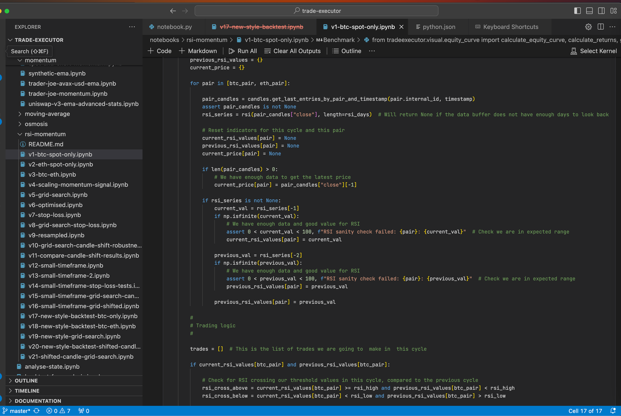
v1: BTC only
In this strategy, we start with Oddmund Groette's earlier RSI momentum trading idea. In his research, he compares using RSI for both mean-reversion and momentum trading for Bitcoin
At this stage, we replicate Groette's research in a Trading Strategy Framework notebook.
The strategy trades
- Buy: RSI crosses over 70
- Sell RSI: crosses under 30
- RSI length: 5 days
Without much thought, we have less drawdown but less absolute profit compared to just buying and holding Bitcoin. Risk vs. reward is good if you ask anyone from traditional finance, but not great if you consider how much the underlying asset has appreciated.
v2: ETH only
We take the v1 strategy and switch the trading pair from BTC-USDT to ETH-USDT.
It becomes obvious that there are some differences in market microstructure between these pairs, and the strategy does not work for ETH unaltered.
v3: BTC and ETH
In this version, we combine trading both BTC and ETH using the same RSI threshold levels.
This is the most primitive version of the portfolio construction system. We do not have a proper signal to help us compare the likelihood of different assets going up or down in price. Instead, we use binary 0 and 1 signals for BTC and ETH trade decisions. If both signals are on, we rebalance 50% / 50%. Read more about portfolio construction in our earlier blog post.
Having two different assets to trade already vastly improves the strategy performance.
v4: BTC and ETH flexible rebalance
Taking the earlier rebalance idea, we set a dynamic rebalance signal. BTC and ETH entries are still triggered by event-driven RSI cross-overs. However, when BTC and ETH positions are open simultaneously, the amount between these positions is dynamically adjusted.
We use ETH/BTC price RSI as the adjustment signal. The theory behind this is that if ETH/BTC has momentum, ETH goes up against BTC, we should hold more ETH in our portfolio. Furthermore, we adjust this signal with an exponent to make it more powerful.
We observe a slight increase in the portfolio performance.
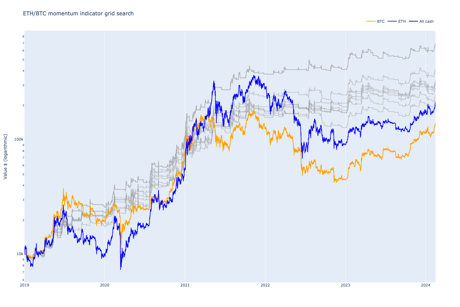
v5: grid search
We run a first grid search to find more optimal parameters for RSI length and RSI cross-over thresholds.
The initial grid search space looks as the following:
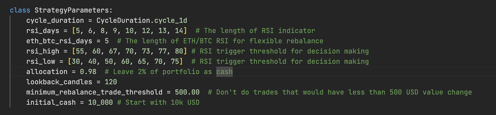
We plot different equity curves for different RSI high and low threshold levels and RSI lengths. With some luck, we can already find strategy parameters that would have outperformed ETH in absolute terms.
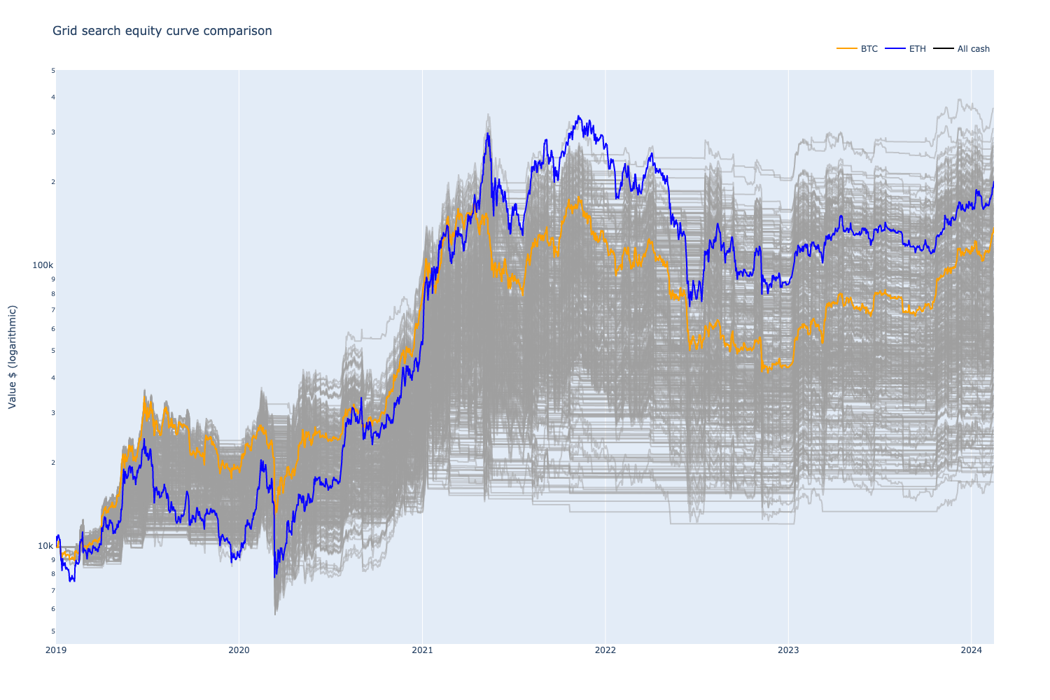
However, by observing the equity curve and trade statistics, we see that with these strategy parameters, the strategy made few trades, was more likely driven by luck, and has yet to show good performance in recent years.
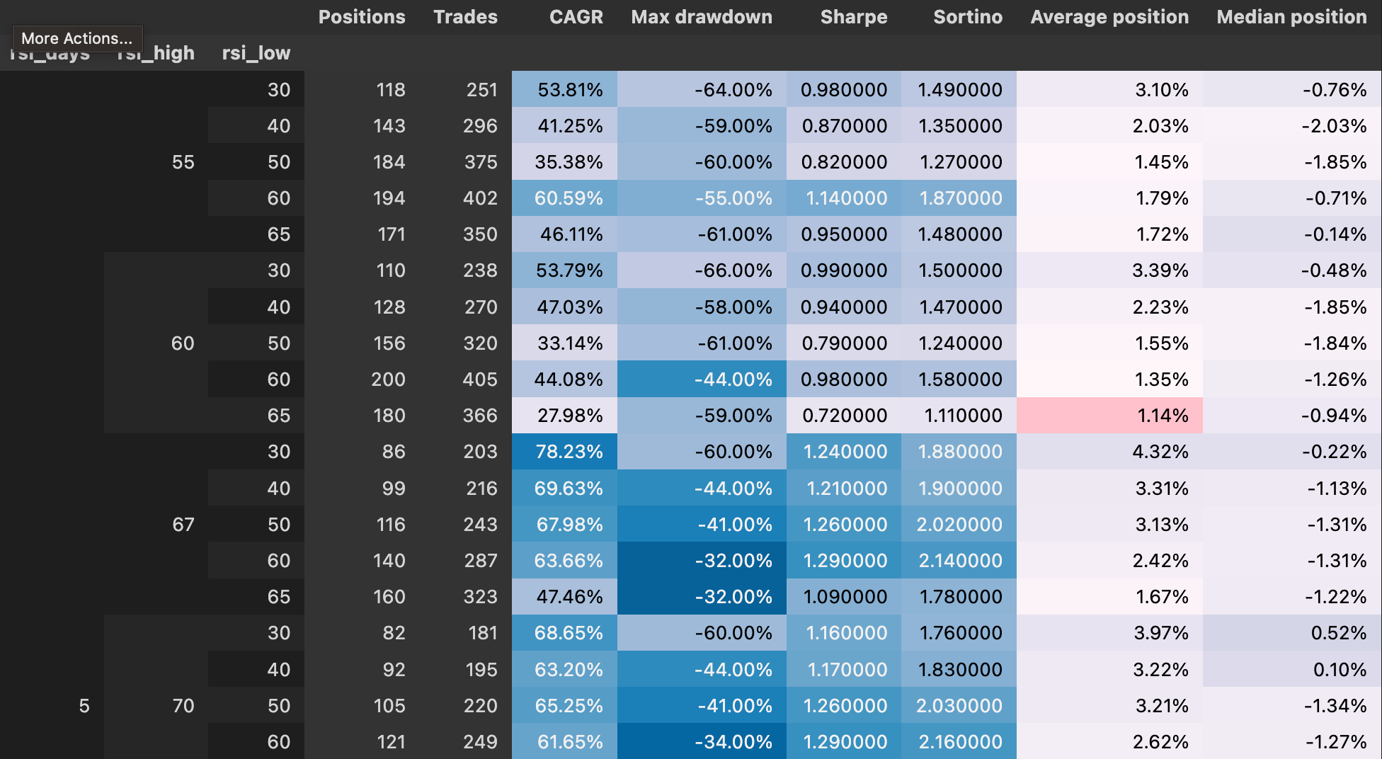
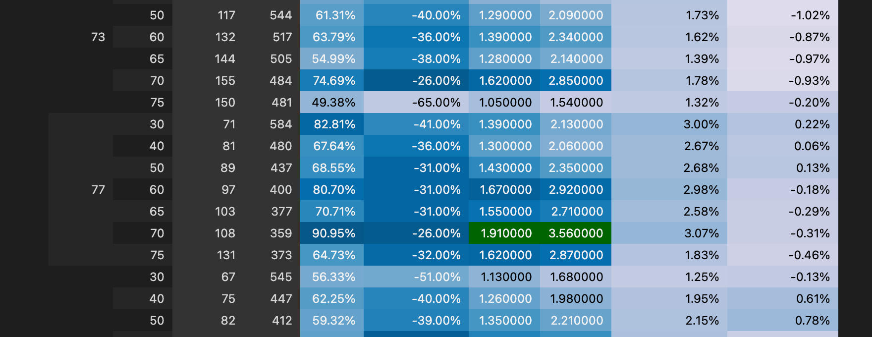
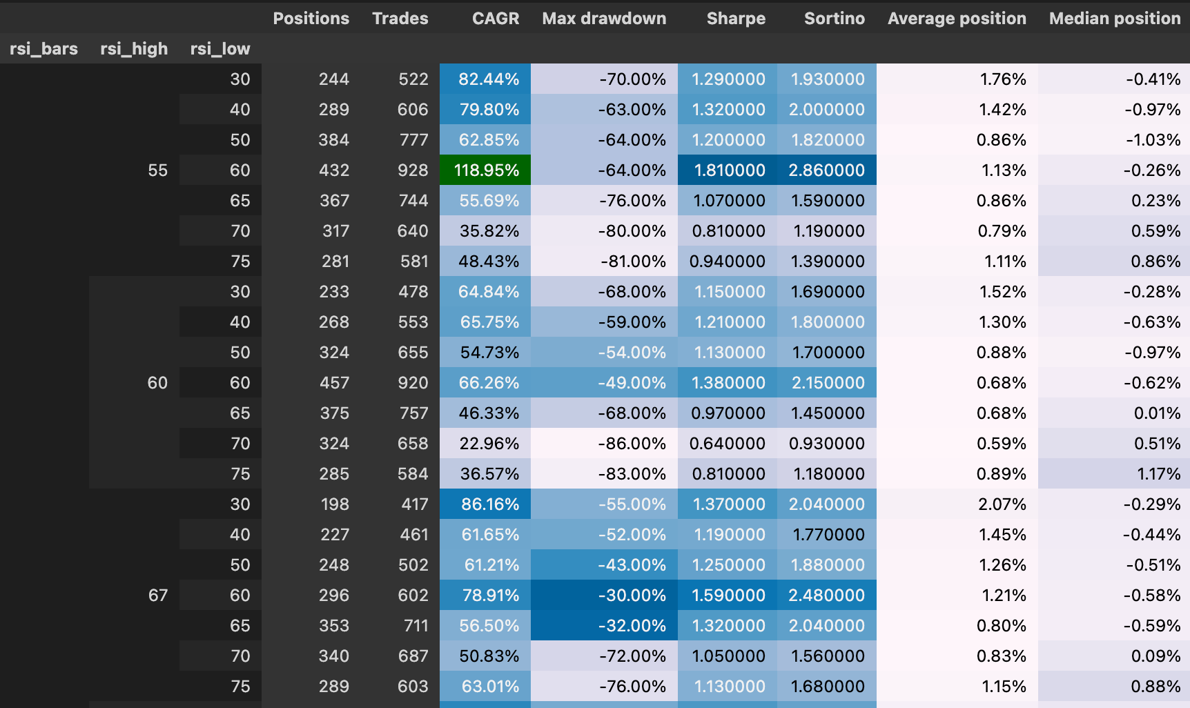
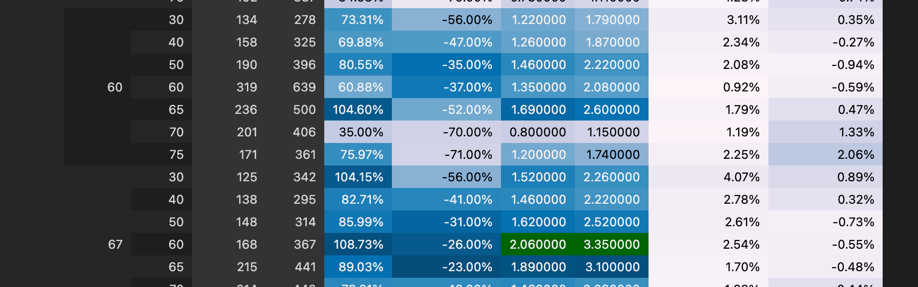
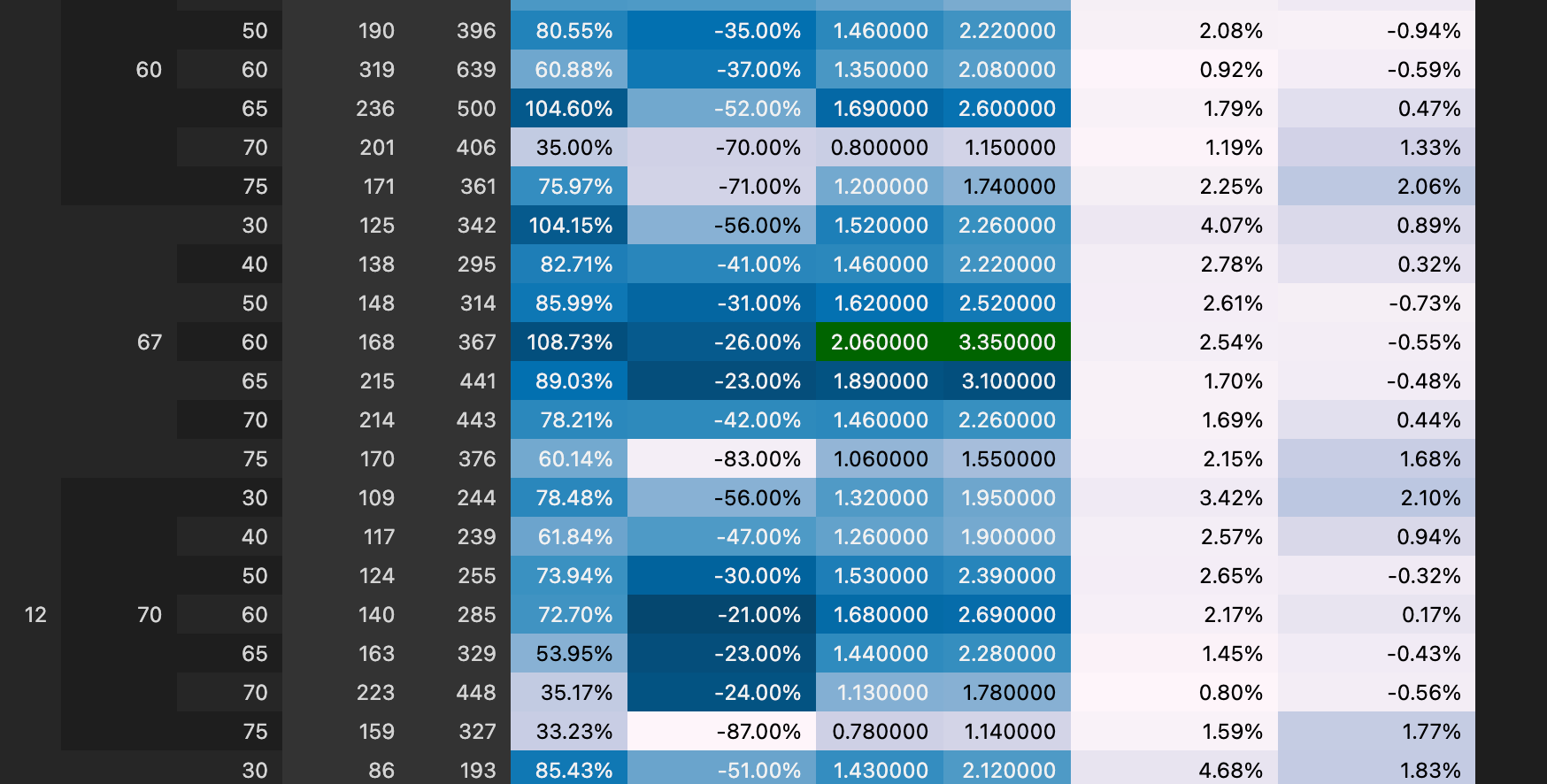
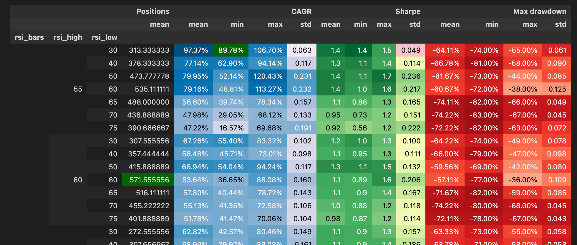
For better understanding, we break down grid search results into a colour-coded table.
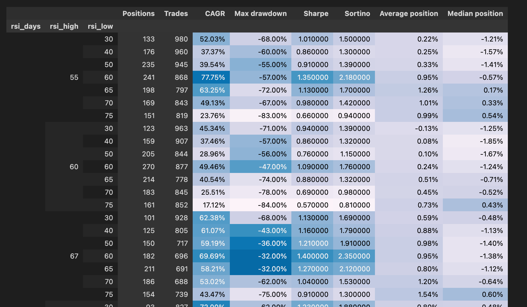
By manually examining the table we find some good candidates for further research.
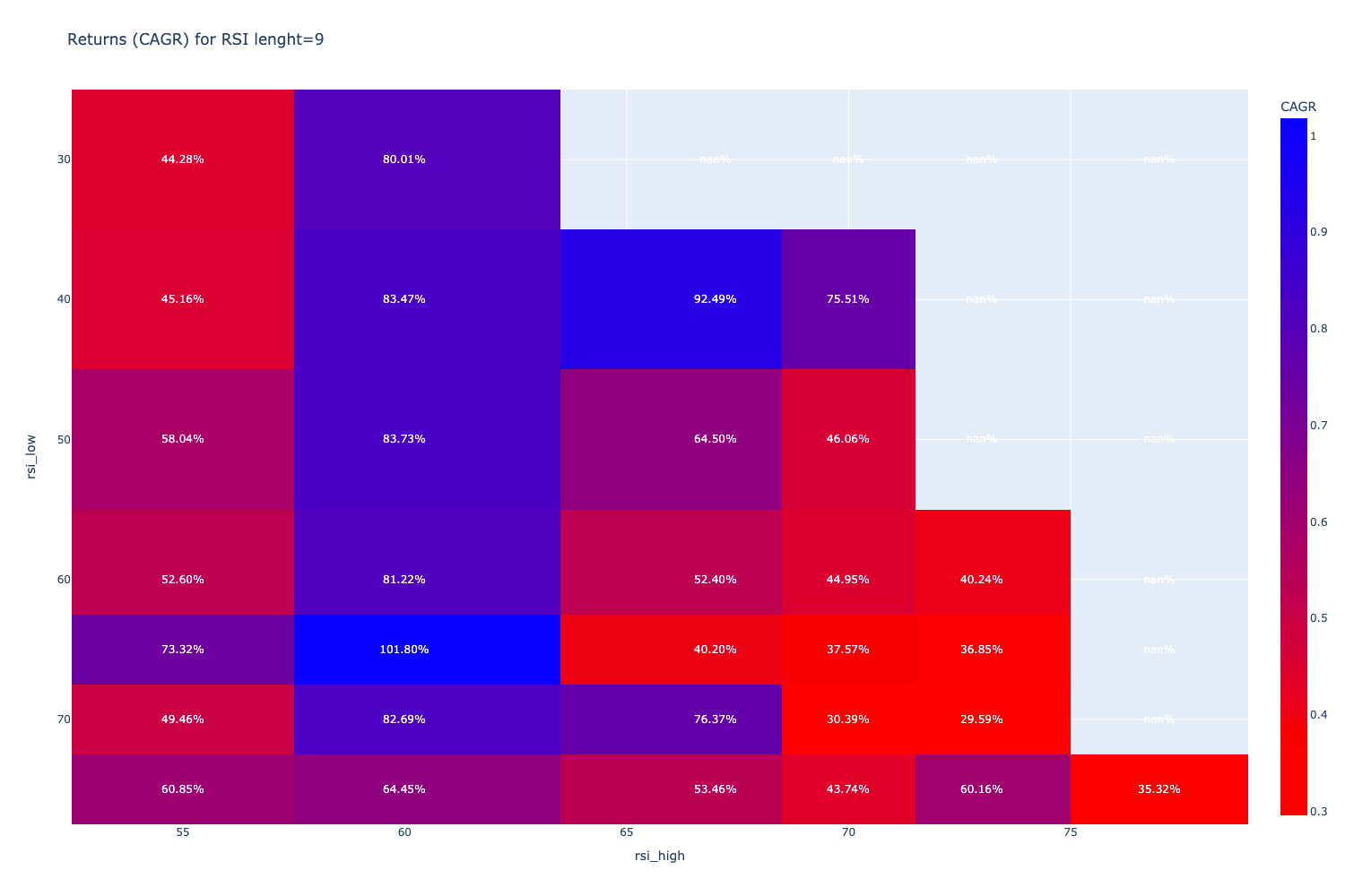
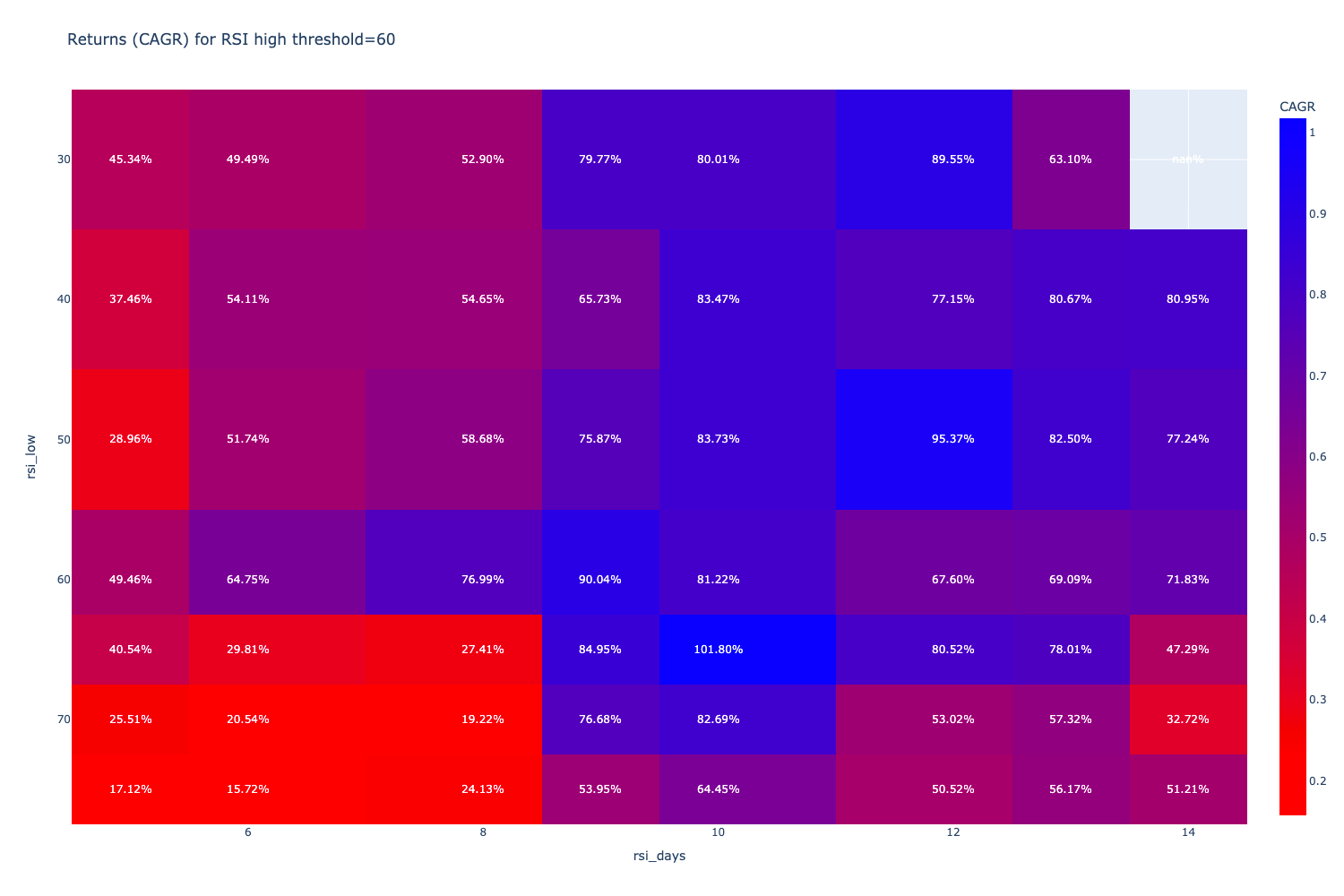
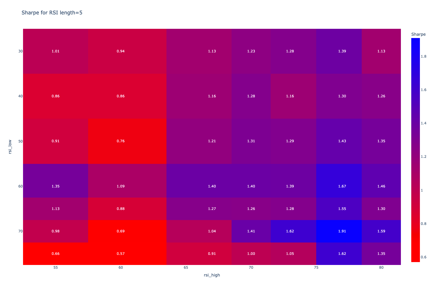
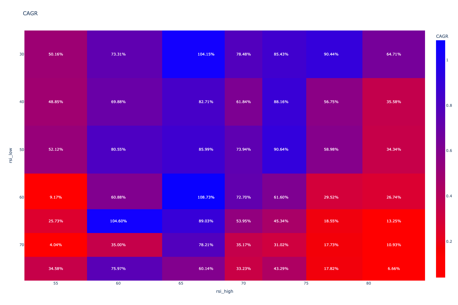
We further break down hotspots in the strategy to 2D heatmaps. Because we are grid searching three different parameters, we need to lock one of the parameters manually for the heatmap visualisation. We also apply a filter and discard results that did only a few trades - we assume these results were more luck-driven.
For functional strategies, the heatmap should clearly show a cluster of better-performing parameters. If there is pure chaos and randomness in these charts, it means the strategy results were mostly randomness-driven, and there isn't likely any alpha.
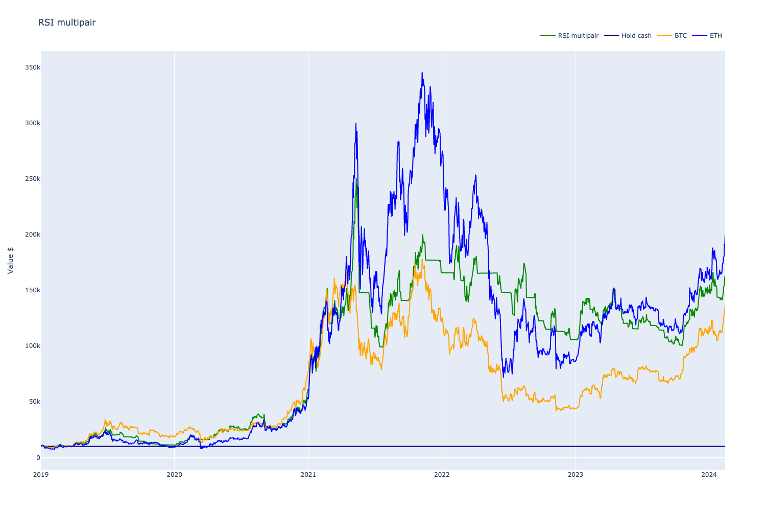
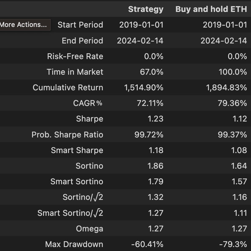
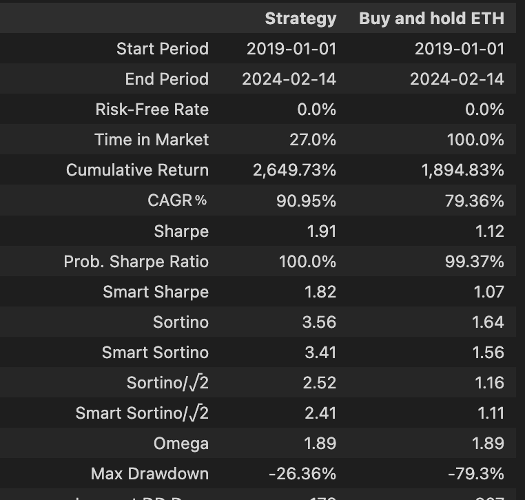
v6: optimised
We picked one of the best grid search candidates and analysed it in an individual notebook. For the “best,” we did not pick one with the maximum profit but one with good Sharpe and Sortino numbers and a fair number of trades.
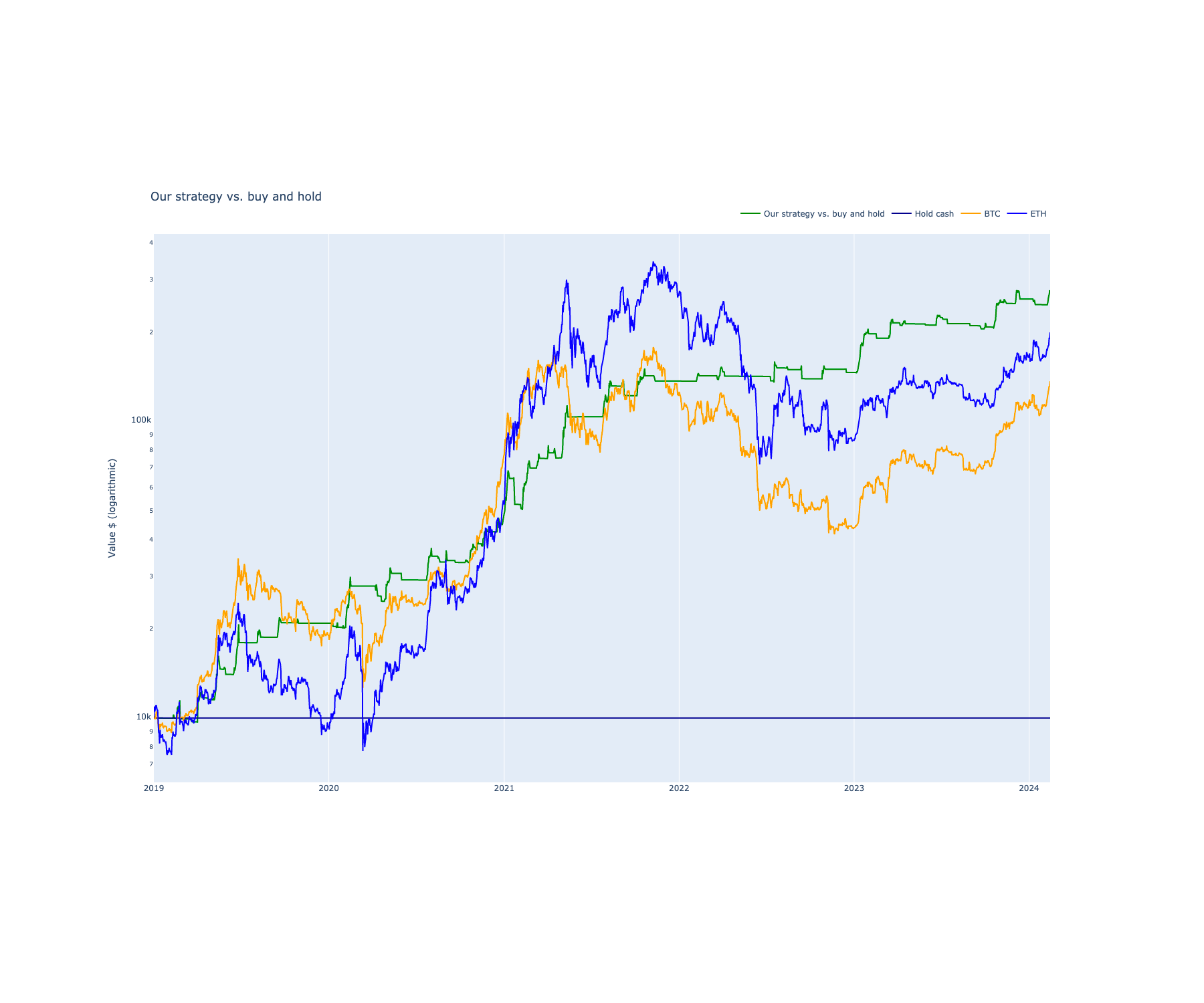
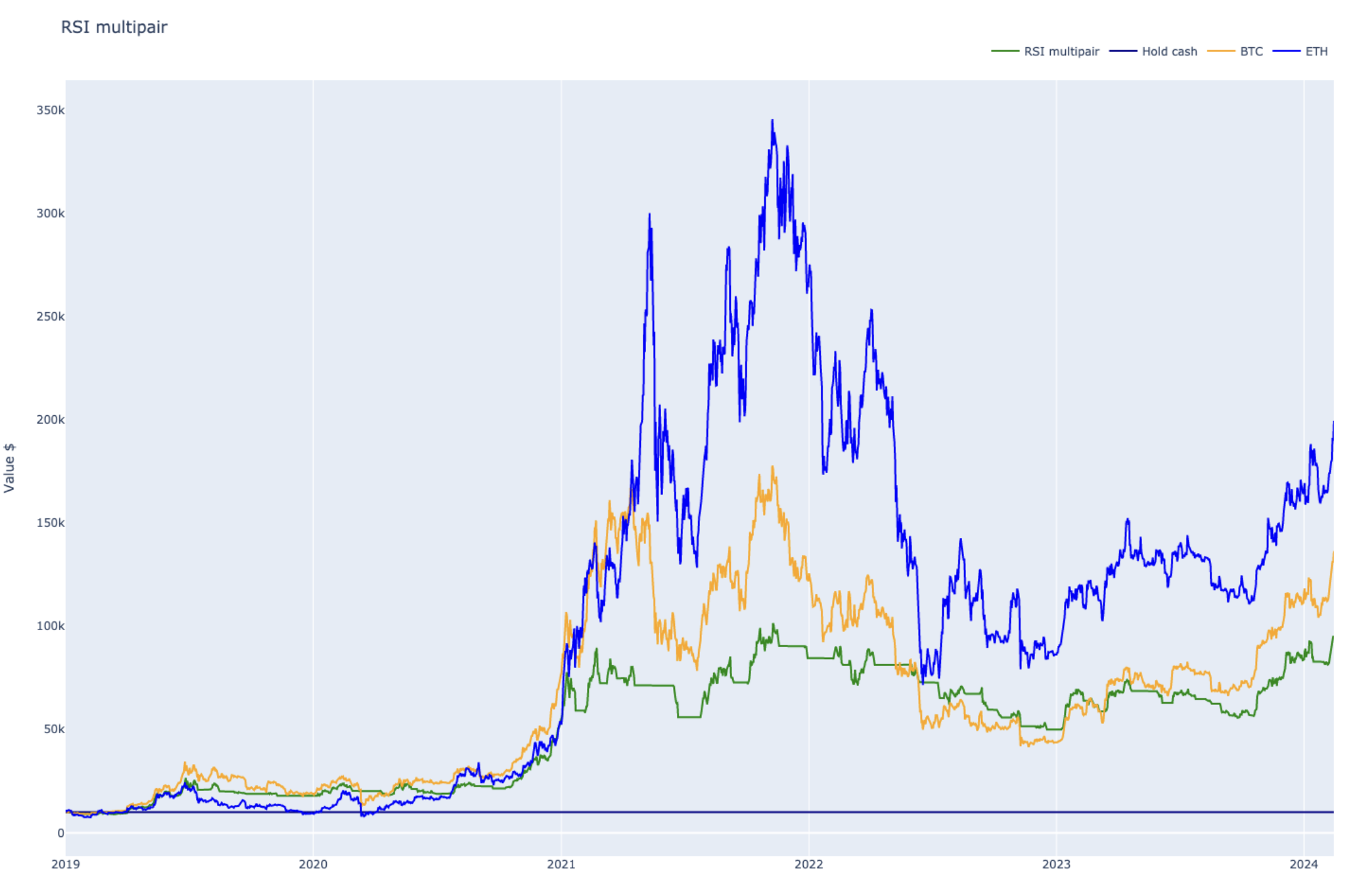
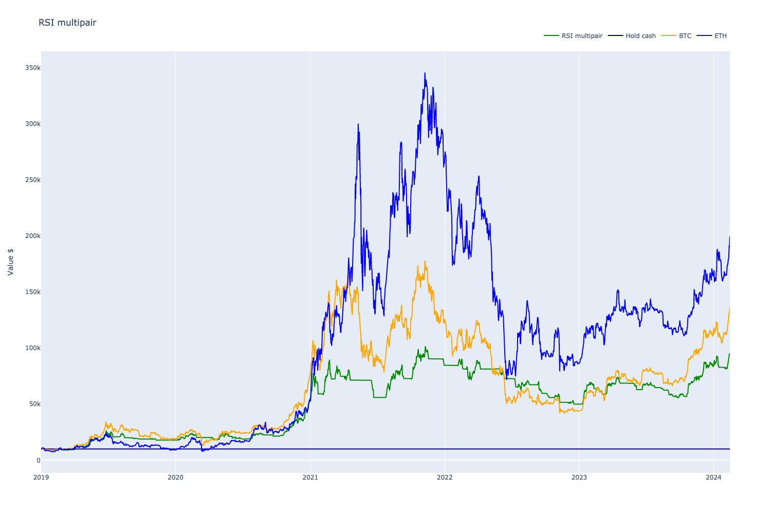
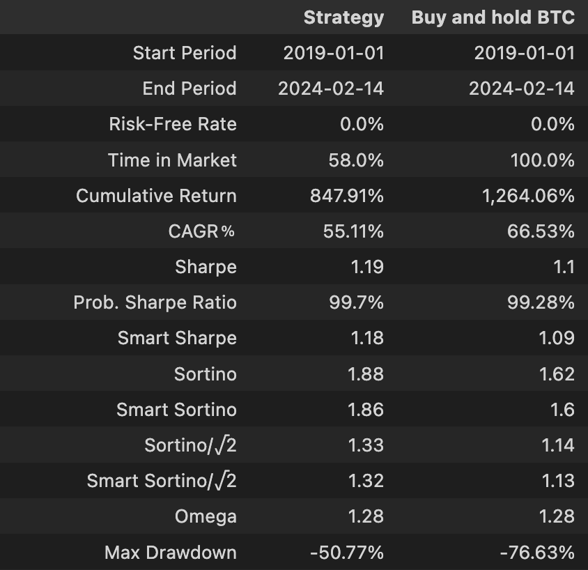
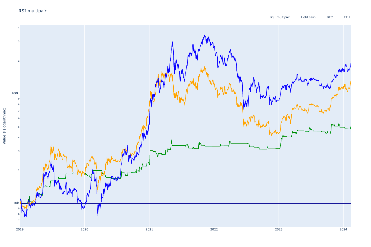
We see that this variant captures fair amount of bull market's upwards momentum, still less than buy and hold, but does not bleed money during the bear market regime.
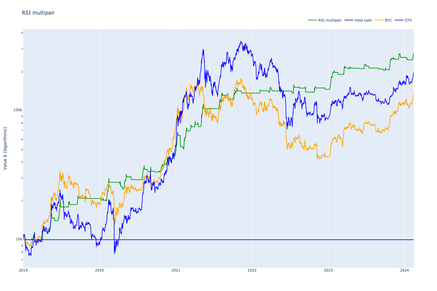
The strategy beats the ETH buy-and-hold portfolio.
Time in Market for the strategy is quite low, less than 30%, meaning that the strategy performance can be vastly improved by having the strategy to do something profitable when it does not hold any open positions.
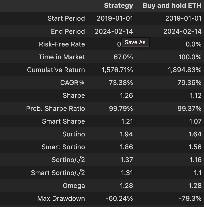
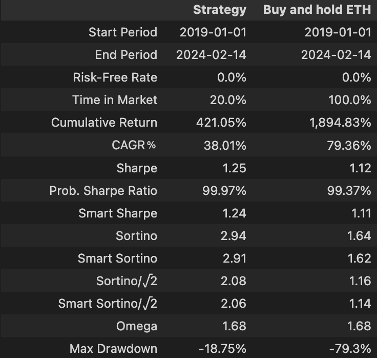
v7: including stop loss
Next, we add a trailing stop to the strategy decision-making process. Our theory is that cryptocurrencies experience volatile drops, and being able to exit the position using stop loss quickly might improve the strategy's performance.
The trade-off with stop loss is that if the stop loss triggers too often, it will also destroy the upside of the strategy, not just limit the downside risk.
The stop loss triggers outside the normal decision-making cycle (1 day). In backtesting, we use a one-hour signal for the stop loss; in live execution, it will be real-time.
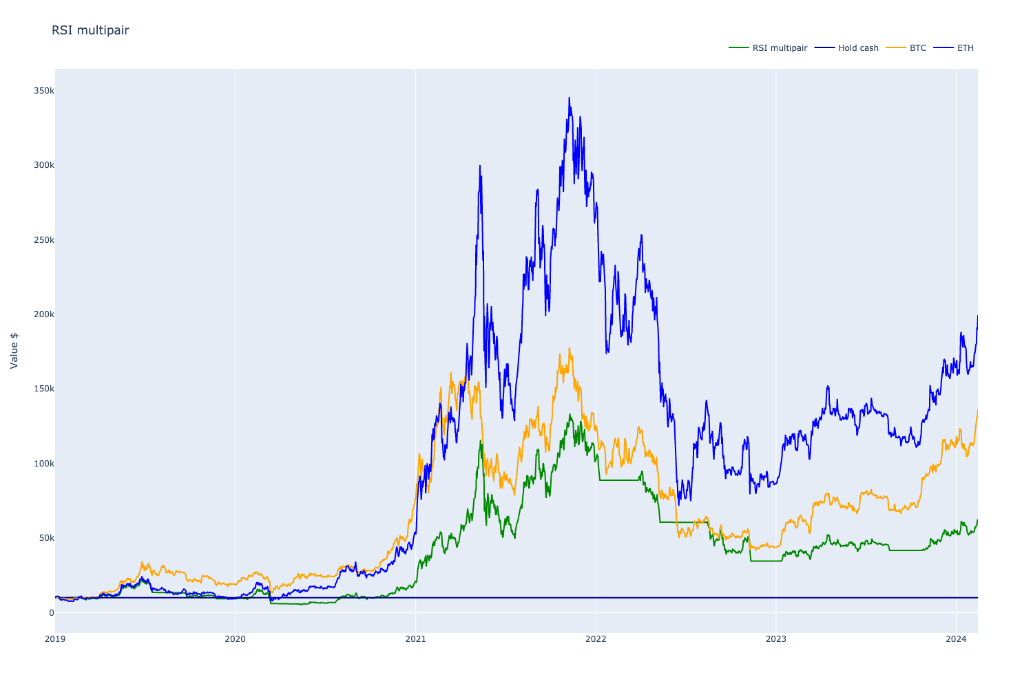
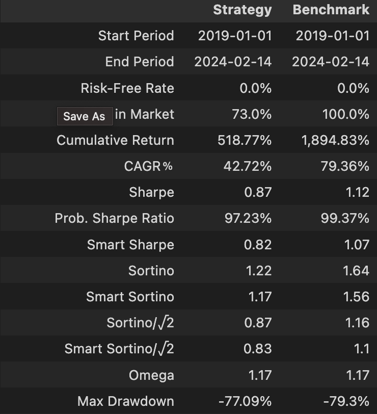
The trailing stop loss indeed significantly reduces drawdown and profits. However the risk-adjusted returns (Sharpe) is still higher for our strategy.
We will revisit the stop-loss parameter search space later in the study.
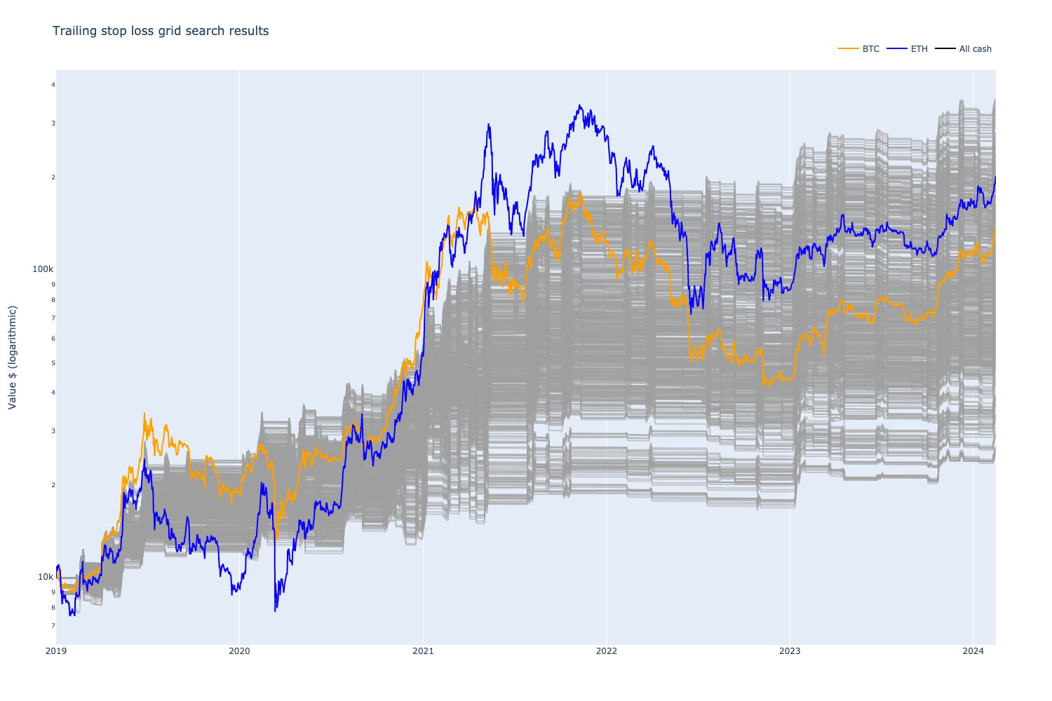
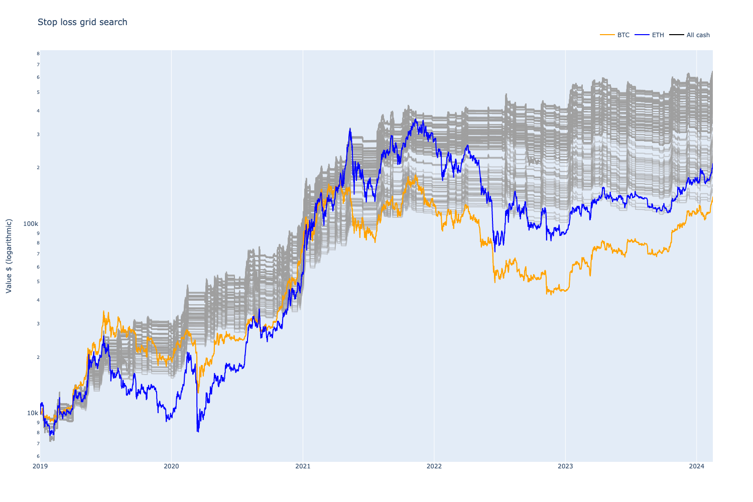
v8: stop loss grid search
We verify whether stop loss can benefit the performance by grid-searching different trailing stop loss parameters. Some minor gains can be made, but in most cases, stop loss does not significantly improve performance and often worsens it.
Note that we limited the search space here by searching fewer parameters than in the previous grid search. We also searched for the ETH/BTC RSI length parameter for the flexible alpha signal.
We used 1 hour close price signal, or interval, to check for the stop loss. In live execution, this would be a real-time price.
We can see some improvement in the results.
If we compare previously searched optimal results with and without stop loss, we can see the effect on Sharpe
We also find some new profit clusters at ETH/BTC RSI length = 20 and stop loss 12.5% values.
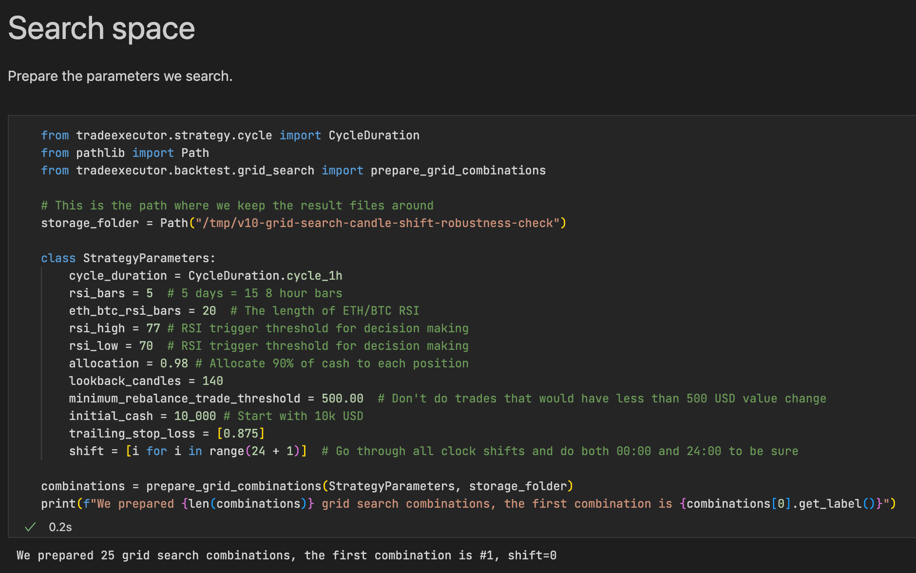
v10: clock-shifted trading hour robustness check
We want to find ways to verify if the strategy performance is luck-driven, or if the underlying trading principles are more solid.
Usual ways to test this are
- Using a different piece of time-series data to train and validate your model (popular in AI)
- Synthetic data: fake data that looks like market data
- Monte Carlo simulations: run your trading algorithm against random or randomised market data
In our case, we do something a bit different. Because cryptocurrency markets trade 24/7, as opposed to 9-5/5 for stock markets and 24/5 for FX markets, the cryptocurrency price feed is continuous. There are no opening and closing auctions in a day. Thus, in theory, there should be no caveats when one trades.
Naturally, this is not completely true. Centralised cryptocurrency exchanges have different demographics (Coinbase US vs. Binance Asia), creating a market microstructure. This is even more true now with Bitcoin ETFs, as ETFs have their net asset value calculated 4pm New York time, creating an arbitrage opportunity.
For our purposes, instead of synthetic or random data, we shift the price feed candles around the clock. Because we are trading daily candles or 24h candles, we can choose a starting clock hour between 0…24. Both 00:00 and 24:00 are included to ensure we did not mess up something in our backtest setup, and the results should be identical.
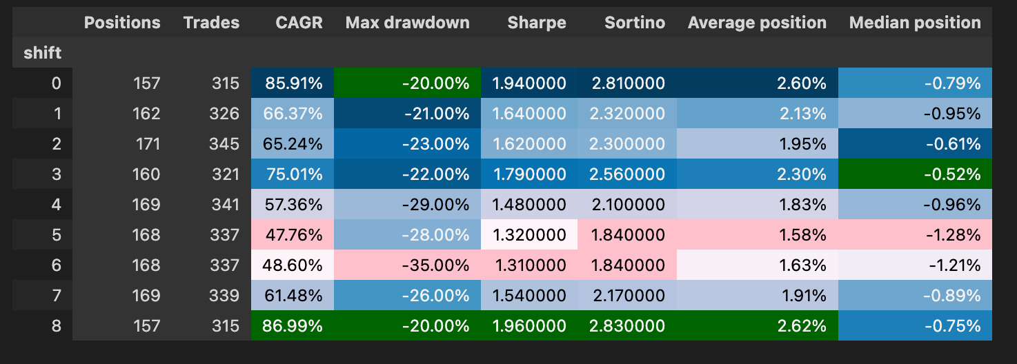
We perform a grid search over shifted trading hours.
We find that 00:00 UTC brings the maximum profit for the strategy, as expected, as we grid-searched for these particular RSI thresholds. However, outside the preceding hours 22:00 and 23:00 the strategy performance degrades significantly.
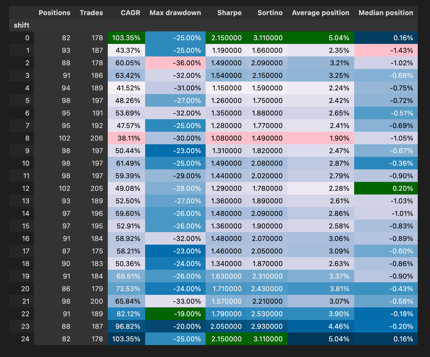
Overall, the variance in the performance is too wide, and further research is needed. Either the strategy is overfitted (likely as there are only ~17 positions per year), something is wrong in our backtest set-up (less likely but possible as this is not a much-explored topic), or we do not understand the market microstructure (something magical going on with certain trading hours).
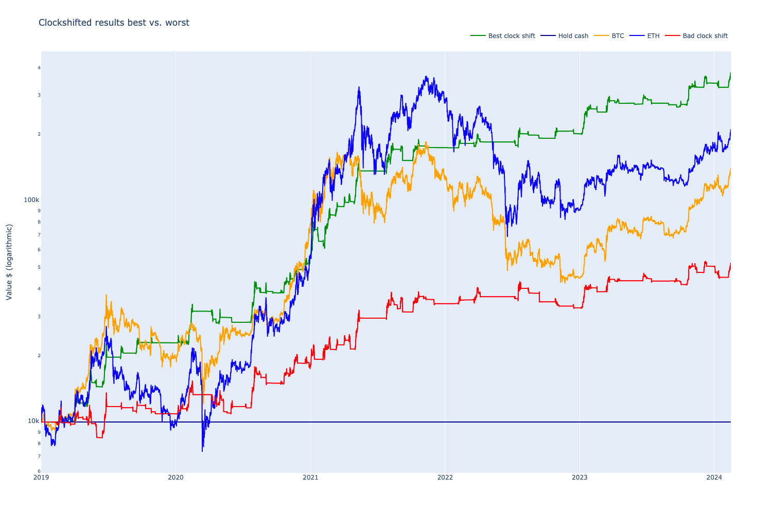
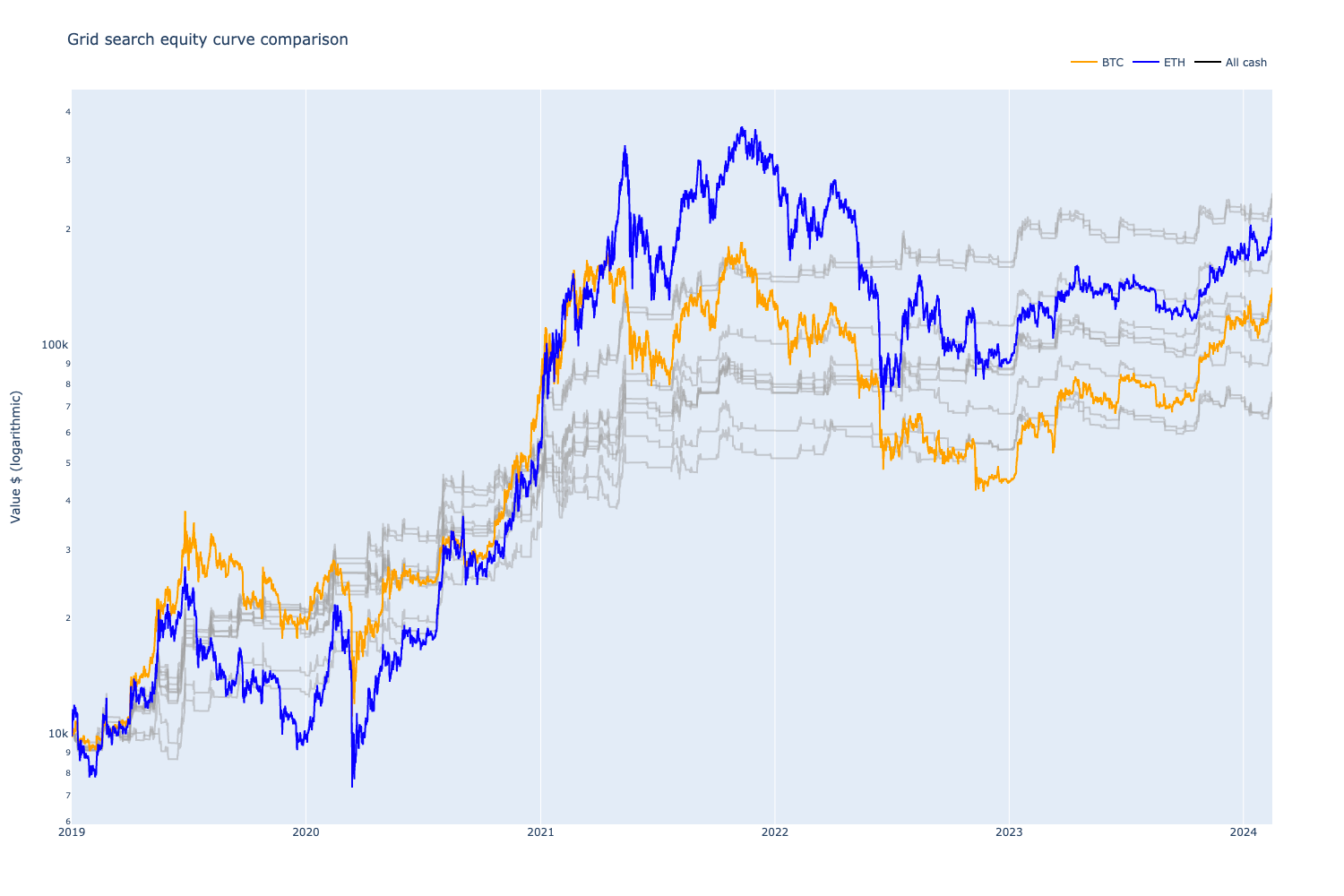
v11: comparing the best and worst clock-shifted result
In this notebook, we take the best (00:00) and worst (08:00) results from the clock-shifted grid search. We plot both equity curves and benchmark these strategies.
The equity curves follow each other, but one makes more profit. Furthermore, the worst option has the profit of buying and holding BTC but with less drawdown.
v12: 8h time frame grid search
In an attempt to make our trading strategy more predictable, we switch from daily (24h) candles to 8h candles. This is possible, because cryptocurrency markets are 24/7 and continuous, as discussed earlier. Our theory is that
- A smaller time frame should generate more profits, as it finds more opportunities
- Shorter and non-standard timeframe should be more predictable and should be more immune to the market microstructure that is related to the daily timeframe
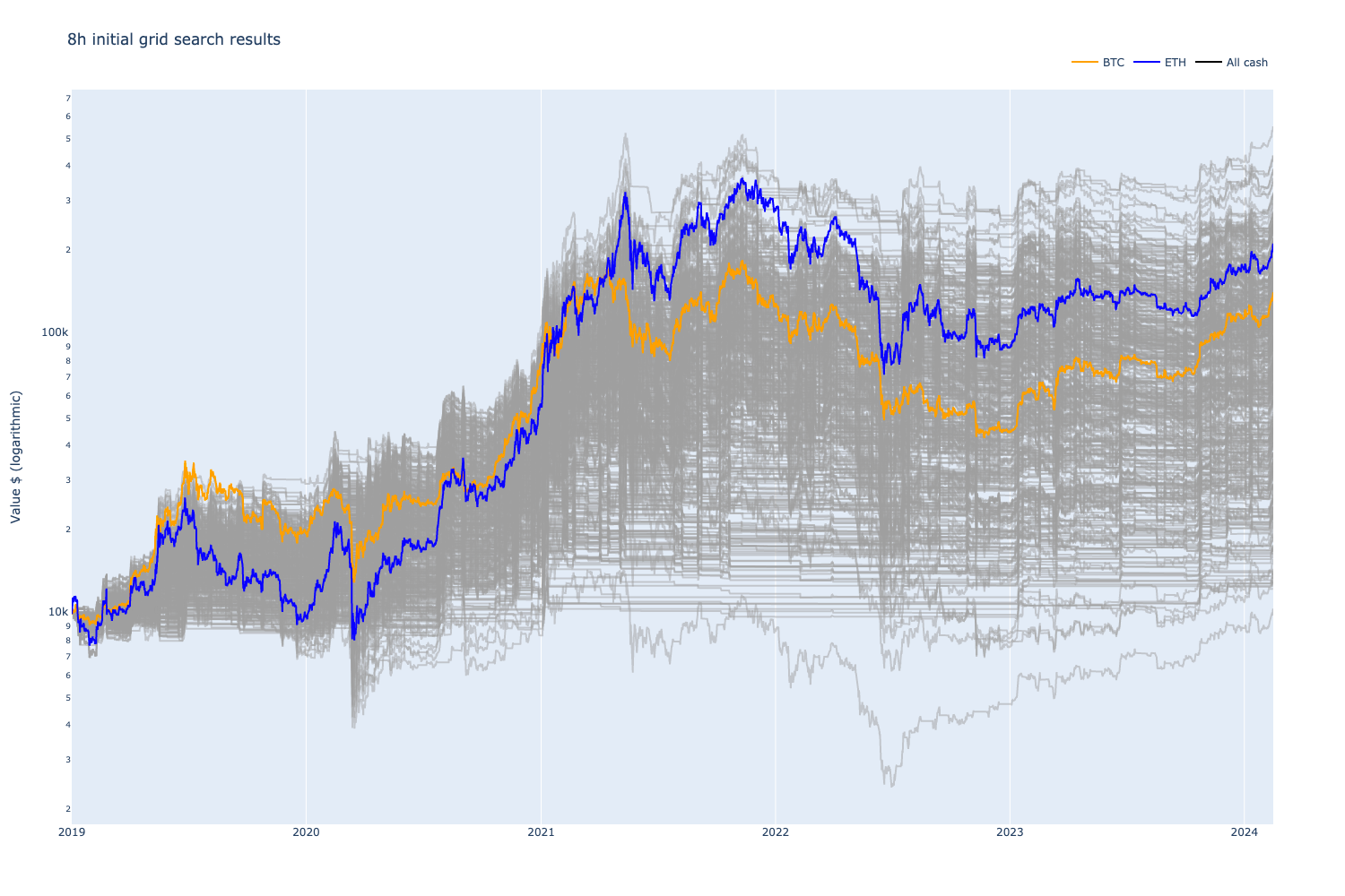
We grid search for the 8h strategy parameter starting point.
Our primary goal, making the strategy open more positions and increase Time in Market, seems to have been accomplished.
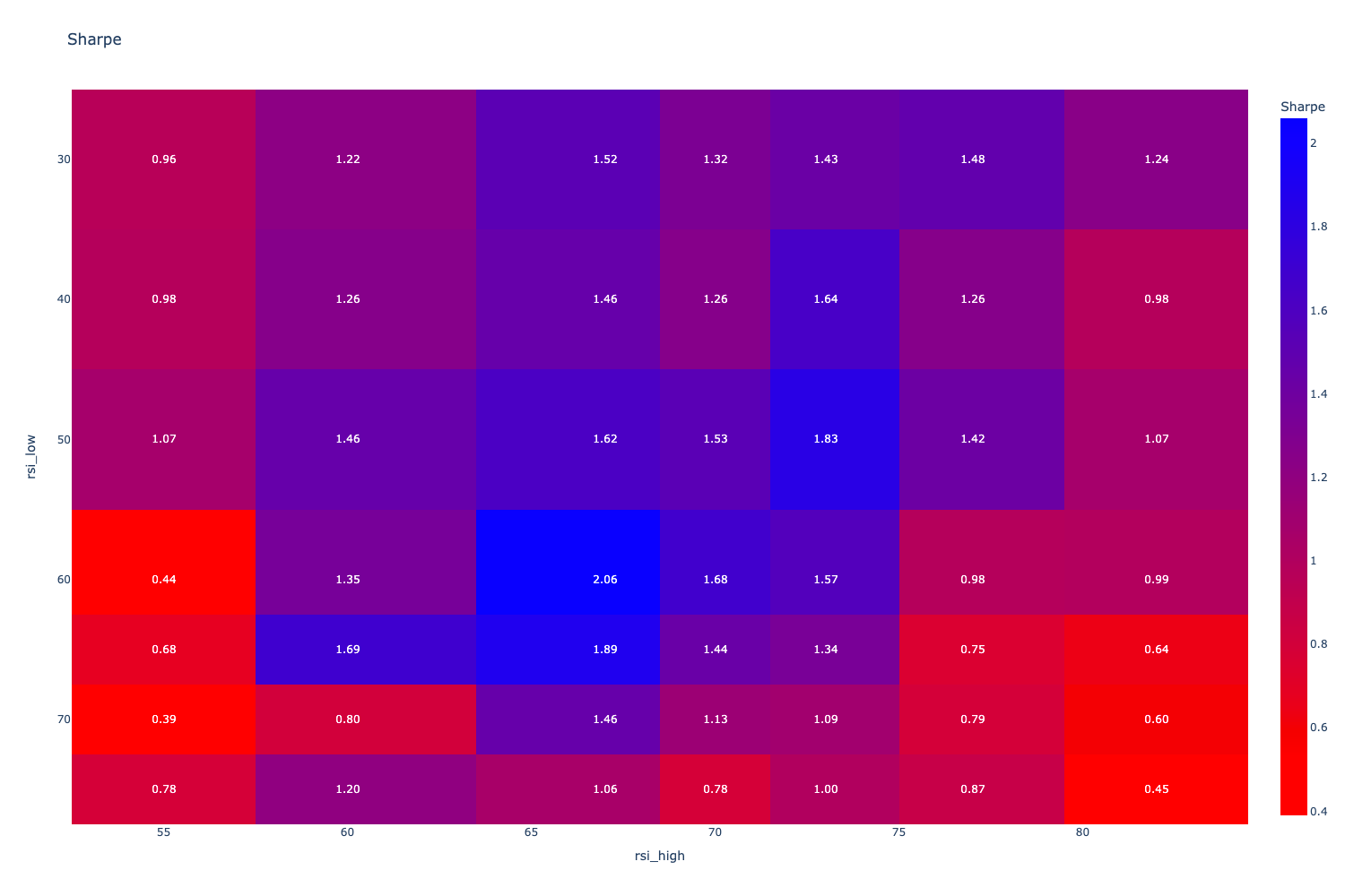
There are some really promising Sharpe numbers.
We visualise 2d heatmaps to understand the grid search results better.


v13, v14: more 8h time frame grid search
We searched for the various strategy parameters, including adding the stop loss. Some of the parameter combinations considerably outperform ETH.
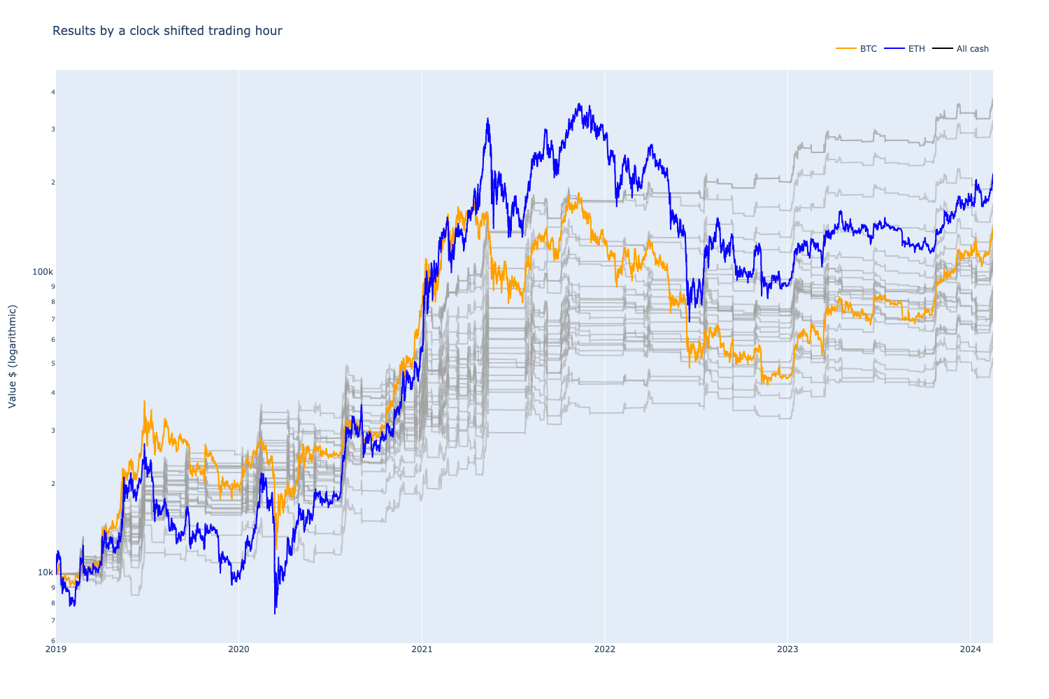
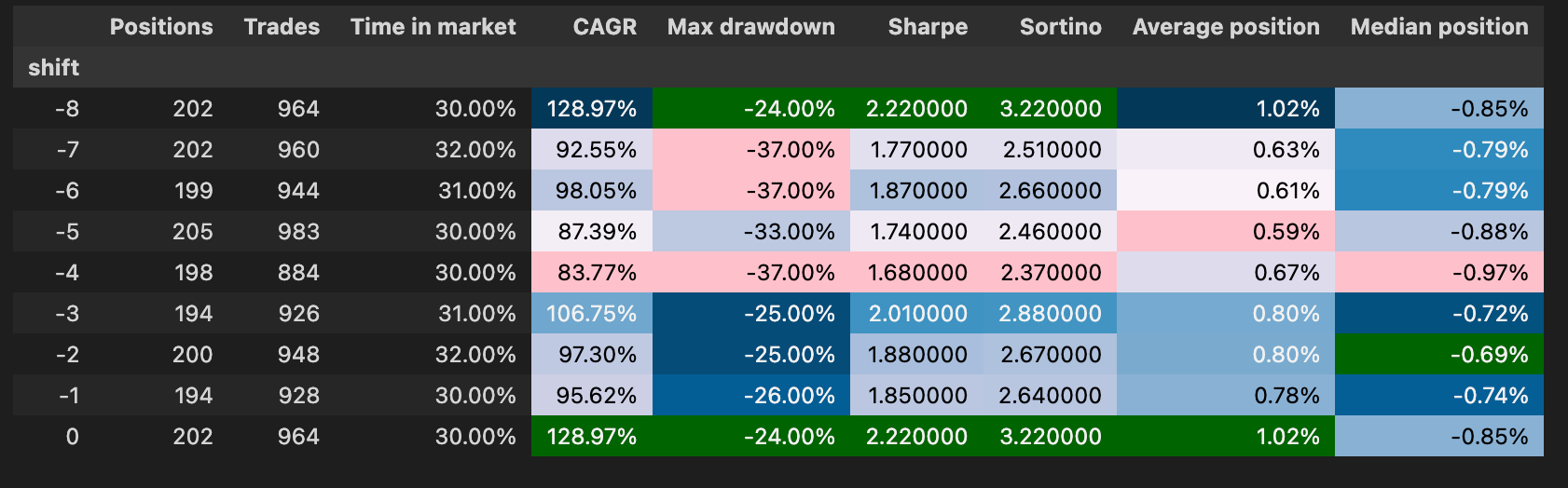
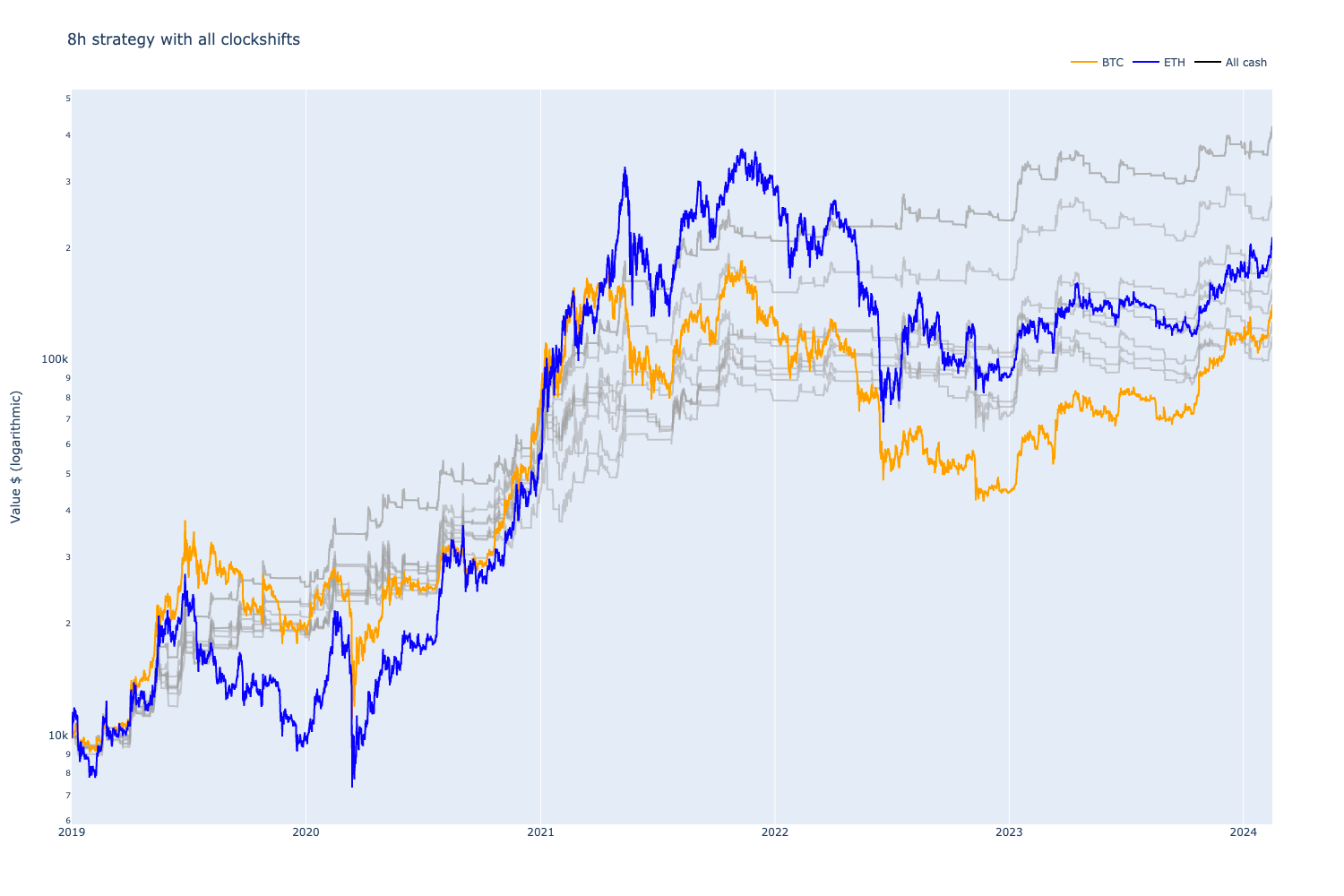
v15: clock-shifted trading hour robustness check
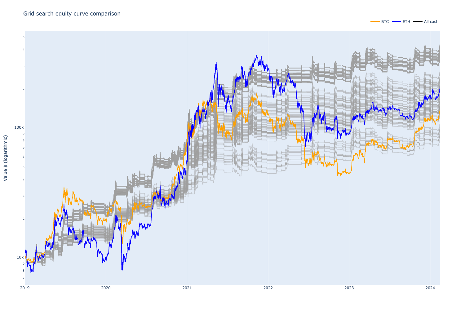
As with the daily candle strategy, we do a clock-shift test by shifting the 8h candle starting trading hour between 00:00–08:00.
Our theory is correct, and the results are more stable than clock-shifted results with 24-hour candles.
The best-performing 00:00 equity curve outperforms ETH, both absolutely and risk-adjusted, using grid-searched parameters optimised for this historical data. Most equity curves land between buy and hold BTC and ETH profit, but the drawdown is much more modest -20% to -35% compared to 70% and 80% drawdown with buy and hold.
Although the drawdown is stable, there is still a lot of variance in profit, which we hope to address in future iterations.
v16, v17, v18, v19, v20: internal backtesting changes
We rewrote our backtests to use cached indicator data. Each grid search worker runs in its process. Earlier, workers recalculated all indicators for each grid search combination run. To speed up backtesting, we switched to precalculated indicators, where the indicator data is calculated once, stored on a disk and then read from the disk by each backtest run.
This gives us 10x - 50x increased performance for our backtesting.
We completed > 10,000 parameter combination searches over a larger 8h candle search space. This did not give us any new findings compared to earlier.
v21: grid search and clock-shift
In our final notebook, we grid search combined clock-shifted 8h time frames and all RSI parameters.
We want to understand the effects of the trading hours better
- How much variation does shifting trading hours cause
- Are the specific hours that are more profitable
- Is the variation within the tolerance for trading
Because we have multiple grid search results for each trading hour, we can compare if some trading hours are better than others, for all RSI parameter combinations.
There are slight variations by hour, as expected, but nothing is significantly out of the line.
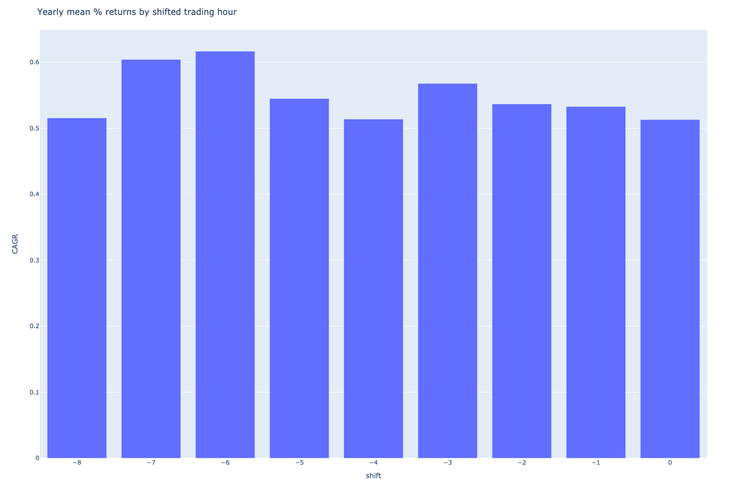
With this kind of grid search, we can compare the strategy performance of each RSI parameter combination, regardless of the starting hour: Are some RSI threshold level combinations more stable than others?
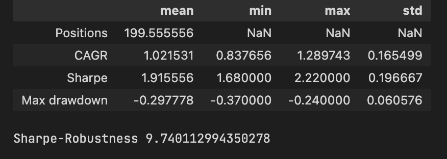
We do this by getting standard deviation (std), min, max, and mean for each RSI parameter combination, as well as all candle-shifted results. The results are then presented in a gradient table. If the Sharpe number is high and the gap between minimum Sharpe and maximum Sharpe is tight, it means the strategy should have more predictable performance characteristics.
Further, to measure the “robustness” of a strategy, we devise our metric. This is not based on any literature but is strictly used in our notebook to rank different RSI combinations against each other. We use the following formula:
Sharpe value / Standard deviation of Sharpe over all time-shifted combinations
Then, we sort out the results based on this number "Sharpe-Robustness" number.
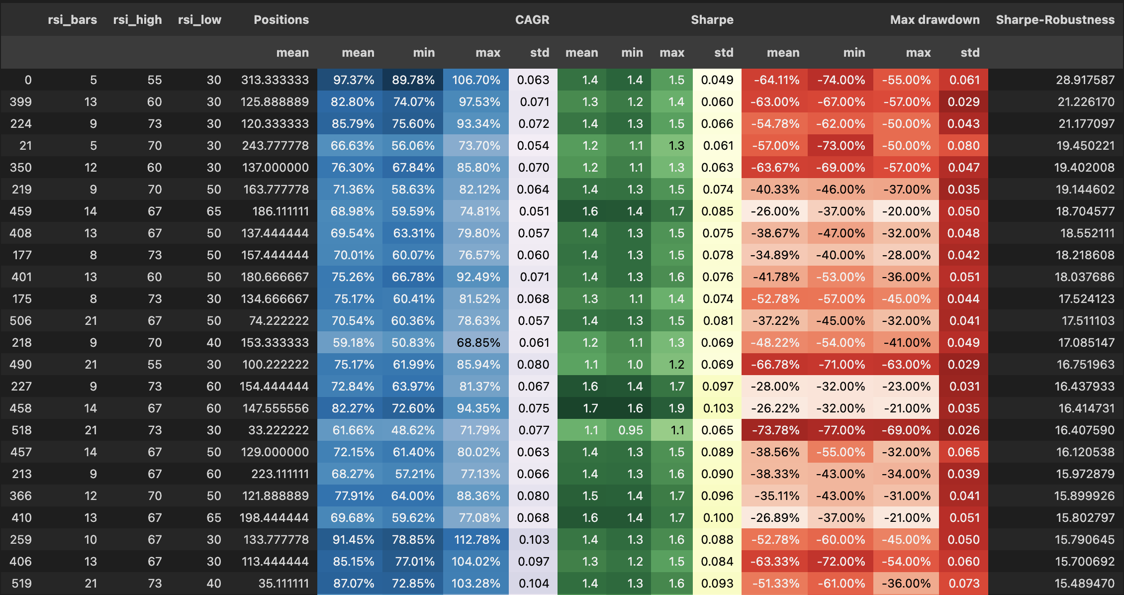
The top hit is a good performer but exhibits heavy maximum drawdown. We also checked the Sharpe-Robustness value of the earlier best parameter combination candidates and saw that they did not deviate significantly from the overall results.
Whether the effects here are statistically significant, we leave for later research.
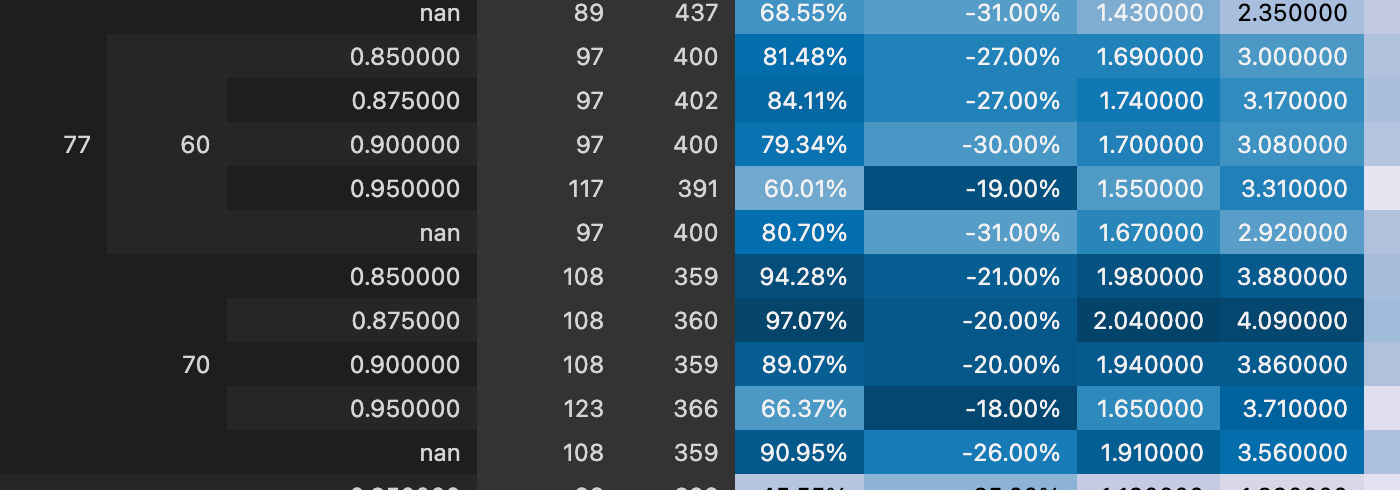
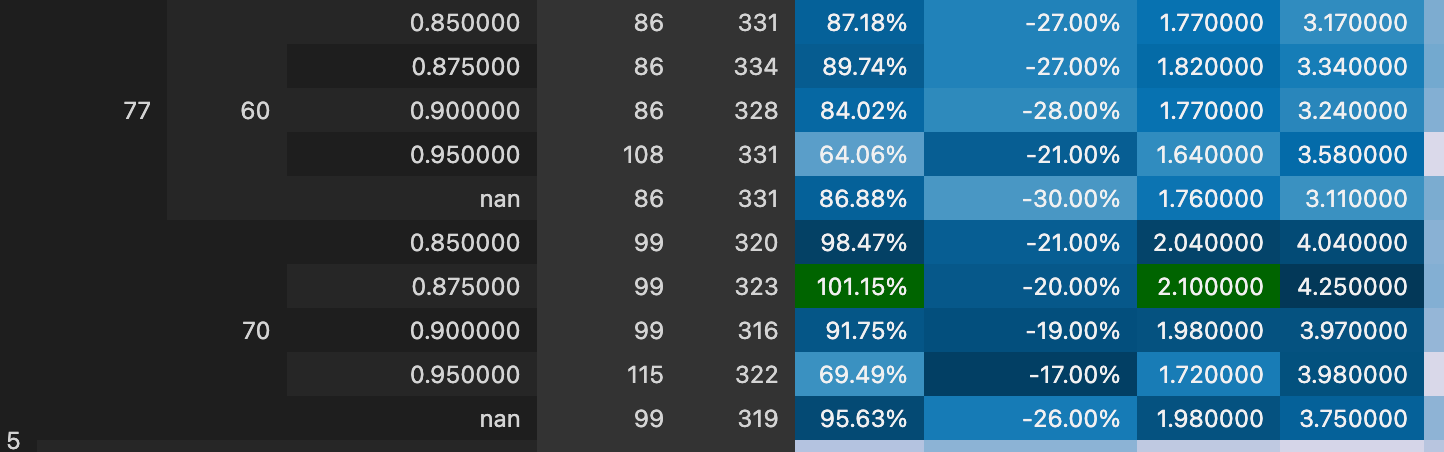
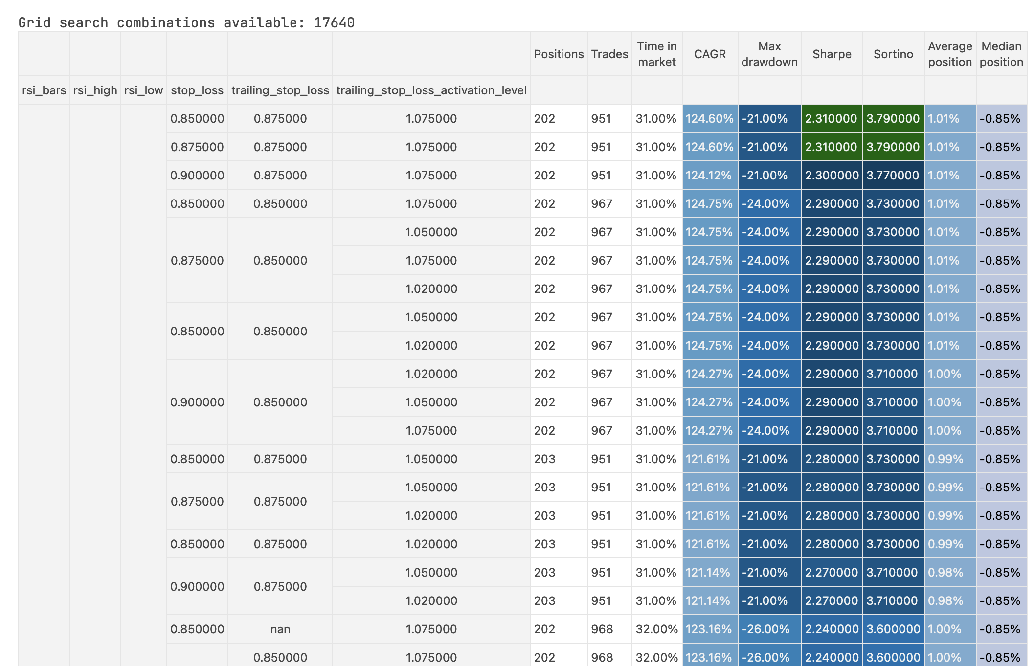
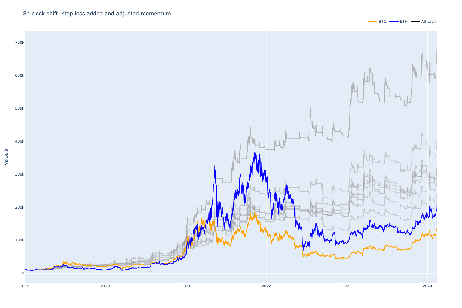
v23 and v24: momentum factor and stop loss criteria grid search
Earlier, we did an initial stop loss grid search but did not end up using this stop loss in the strategy yet. We also did not try to determine good threshold for rebalancing criteria.
In these notebooks, we search
- Stop loss: initial stop loss
- Trailing stop loss: dynamically updated when the price moves up
- Trailing stop loss activation level: how much price needs to move up before we start to use trailing stop loss
- Momentum exponent: the factor of how strongly to rebalance between ETH/BTC
- ETH/BTC RSI length: what is a good duration of RSI to determine the momentum factor
We also reworked the momentum formula to have an exponent factor to search if capturing more momentum gives us any better results:
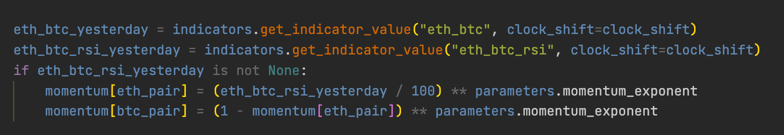
We find that using stop loss, trailing stop loss, and such will improve our performance. We have a profit bump ~100% CAGR --> 120% CAGR and some reduced drawdown.
- Momentum factor: 2.5
- ETH/BTC RSI length: 3 bars (1 day), shortened from the earlier 5 bars
- Stop loss: 20%
- Trailing stop loss: 5%
- Trailing stop loss activation level: 7% up
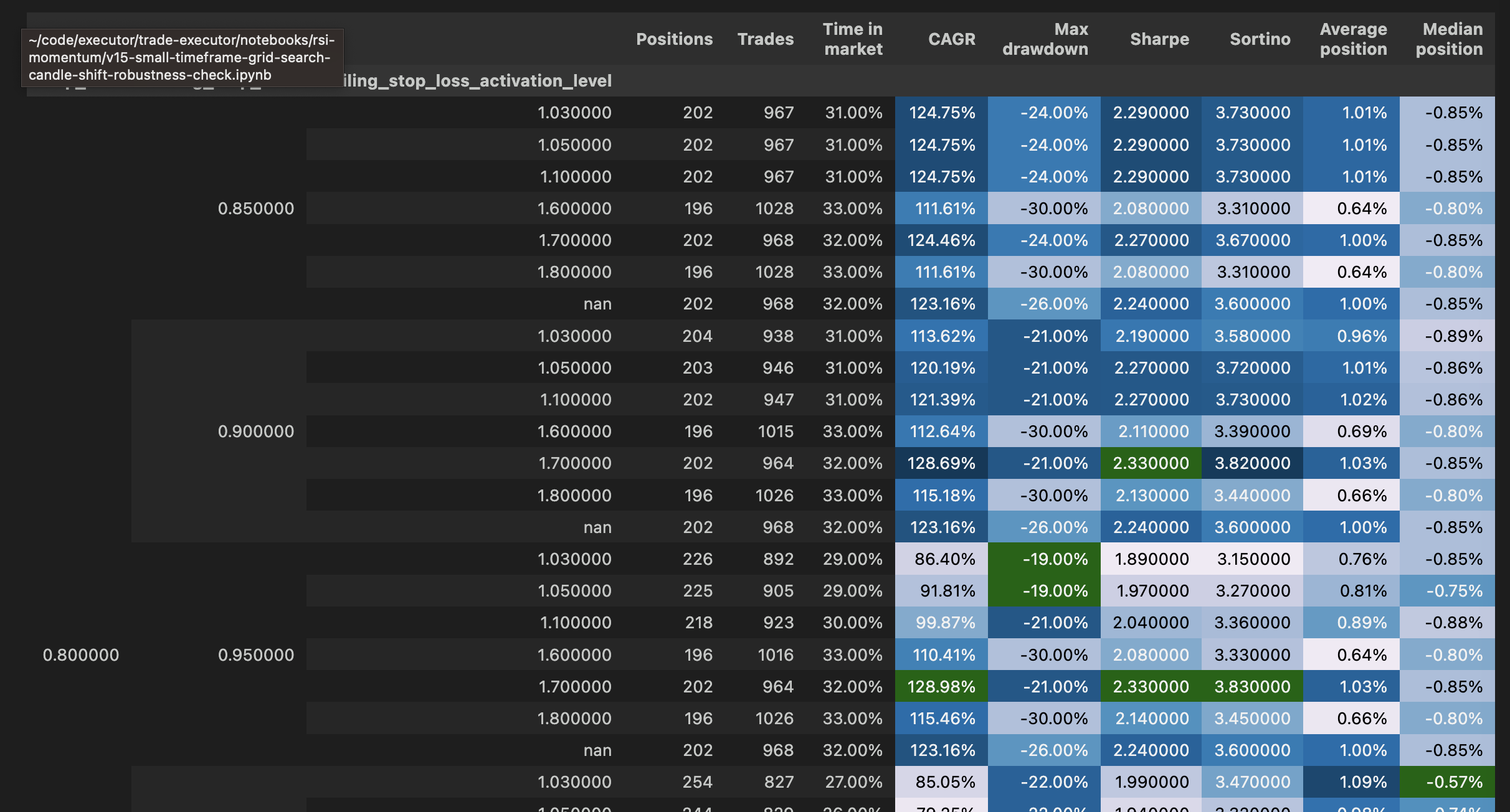
We can see how the stop loss and momentum parameters affect the previous best-fit parameters, giving us some additional gains.
v25: Re-checking robustness with a clock-shifted grid search
Based on the modified stop loss and momentum parameters above, we re-check the robustness of the strategy.
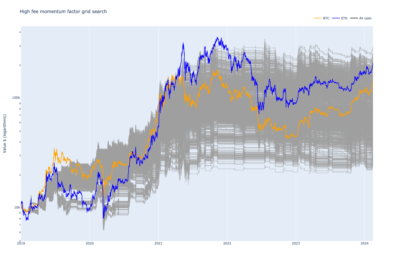
v27, v28: Higher trading fee scenarios
We are trading high-liquidity BTC and ETH pairs. Although trading fees should not be an issue, we want to explore their effects on this strategy.
The above backtests were done using a 5 BPS taker fee without price impact. In decentralised finance, some common fee tiers include
- Uniswap v3 has a 5 BPS fee tier for liquid pairs. Read more in this blog post.
- Uniswap v2 has 30 BPS fee
- PancakeSwap, Uniswap v2 clone on BNB Smart Chain, has a 25 BPS fee
Increasing the trading fee severely affects the strategy performance.
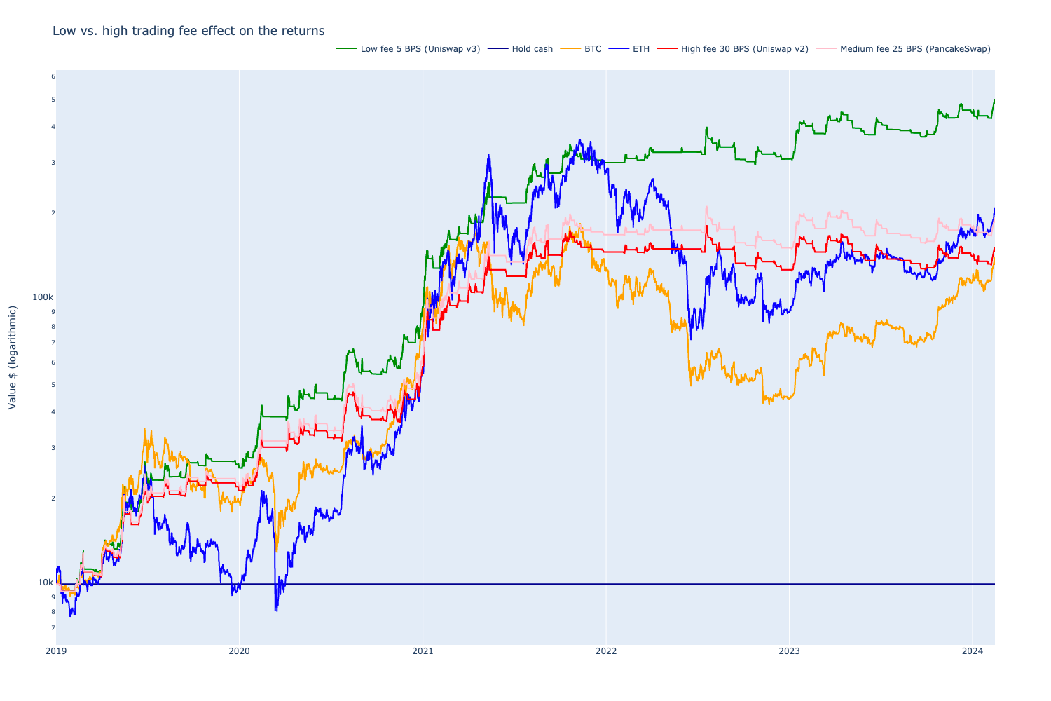
The strategy is very fee-sensitive. The strategy does ~40 positions and ~200 trades annually, so this makes sense. This is typical for simple algorithmic trading strategies.
If we want to compensate for higher trading fees, we can grid search different strategy parameters with higher trading fee settings. We assume that, in this case, strategy parameters that make fewer trades outperform.
Conclusion
In this article, we’ve provided a detailed walk-through of the research process to create and optimise a simple RSI-indicator-based BTC and ETH momentum trading portfolio strategy. For this type of strategy, we can expect to profit somewhere between buy-and-hold ETH and buy-and-hold BTC. However, the strategy profit comes with less maximum drawdown, meaning that the strategy is less risky compared to buy-and-hold.
To present one "chosen" strategy, the following parameters seem to be a good compromise:
- A one-trick pony, using only the RSI indicator
- 8h time frame for OHLCV candles
- RSI length of 12 bars
- RSI high threshold (momentum starts) = 67 bars
- RSI low threshold (momentum dies) = 60 bars
- ETH/BTC Momentum: RSI 3 bars, 2.5 exponent adjustment
- Stop loss 20%, trailing stop loss activation at 7%, trailing stop loss 5%
With the time frame and parameter space we searched, we can expect 40% - 100% CAGR with a 20% - 40% maximum drawdown. Most strategy variants beat BTC buy-and-hold regarding absolute profit and risk-adjusted returns. Sometimes, these simple strategies also beat ETH buy-and-hold in absolute terms. As a rule of thumb, the algorithmic trading strategy performance can be expected to be ~1/3 worse than backtested results because of overfitting, lack of data, change in market microstructure and so on.
The maximum drawdown of more than 20% may be considered risky in trading. This kind of risk vs. reward range might be suitable for cryptocurrency traders, but the maximum drawdown is probably too much for investors from the traditional markets. We can further cap the drawdown, but this starts to eat profit as well.
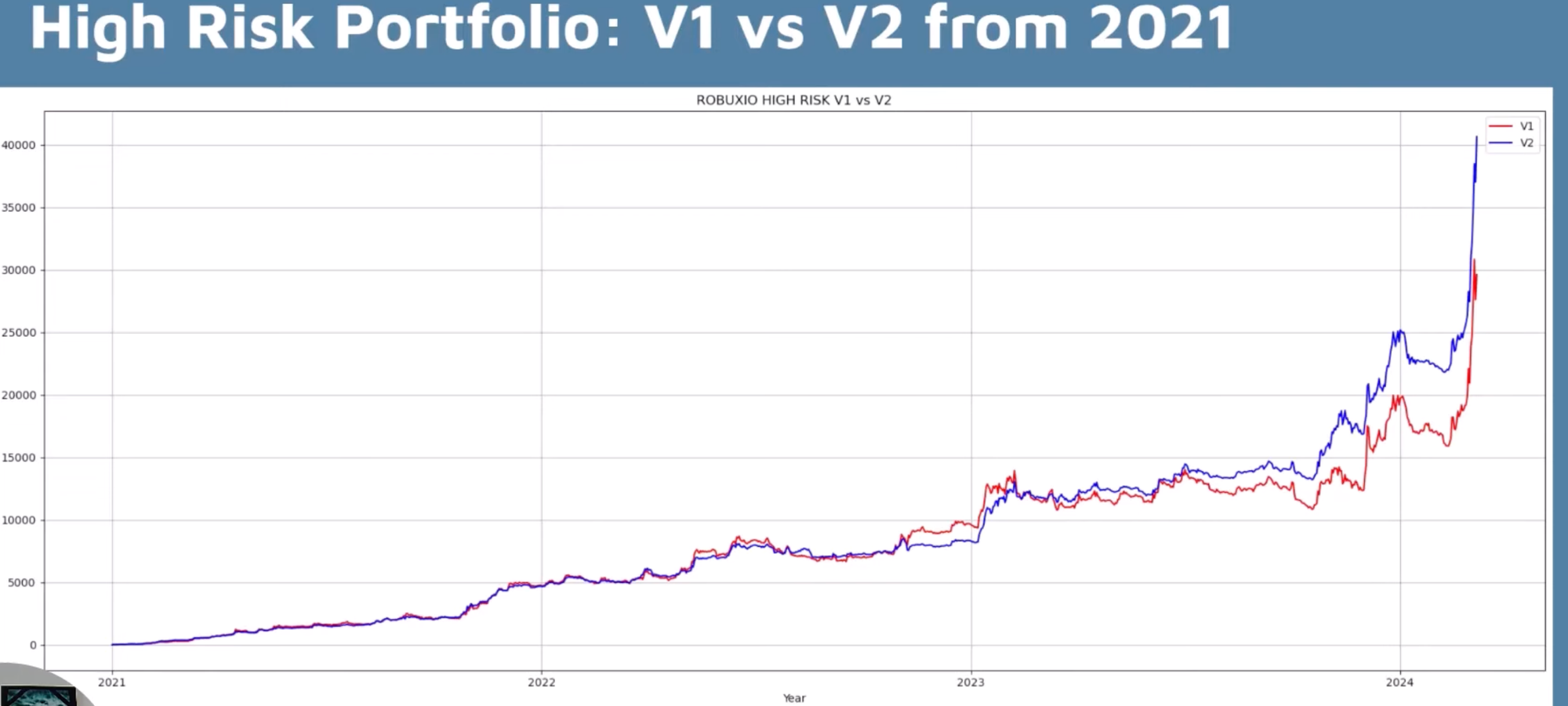
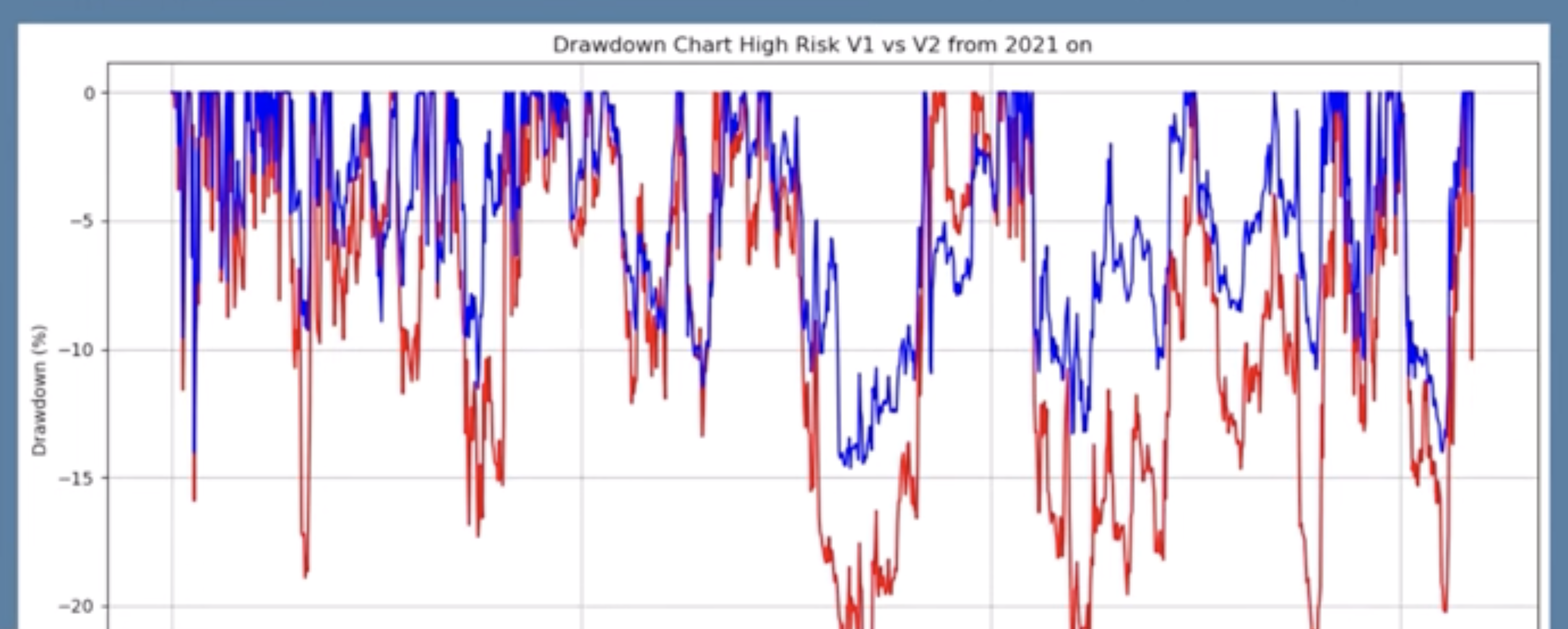
We can also compare our strategy to a professional proprietary trading strategy which is much more complex:
- A proprietary strategy (with new v2 and old v1 variant)
- A high-risk portfolio construction strategy with multiple sub-strategies
- Trades a much larger asset universe than BTC and ETH
- We see that profit is much higher for about the same maximum drawdown
Our simple strategy has a lot of room for improvement. In the upcoming blog posts, we will explore how to improve and build more complex strategies.